Chapter 6 Lesson 31: Numerical Solutions

6.1 Objectives

Understand visually how Euler’s method uses the slope at one point to approximate the next point of the solution a step size away for an IVP.
Given a first‐order IVP and step size, approximate the solution at a specified input (or for a specified number of iterations) using Euler’s method by hand.
Understand that in general the accuracy of Euler’s method is improved by decreasing the step size.
Given a first‐order IVP and step size, use R to implement and/or visualize Euler’s method.
Given a pure‐time first‐order ODE, initial condition, and step size, compare the numerical approximation from Euler’s method to the analytical solution at a specified input in order to compute the error of the numerical approximation.

6.2 Reading

Chapter 6 of the Supplemental Reading

6.3 In class

Analytical solutions not required. Even though we might not be able to compute the analytical solution to an ODE when the functions involved are not integrable, we can approximate solution values using the information we do have (much like we did with the vector fields).
Pick a starting point and a step size. We do need to specify a starting point (initial condition) and how much we want to increment the independent variable for each iteration of the numerical approximation method.
Euler’s Method. The method we are using in this course, Euler’s method, requires you to know three pieces of information: the current approximated solution value, the step size we want to take to get to the next approximated solution value, and the direction we need to step in given our current position. We can calculate the new “current position” and continue computing the next step using an iterative process.

6.4 R Commands

Euler, plotPoints

6.5 Problems & Activities

There are no less than one million ways to motivate Euler’s method. I’ll describe two of them here. Do what works for you.

First, the thing that is most successful for me (Joe) personally is to say “Suppose I’m driving on I-25. Right now my car is at mile-marker 152, and I’m heading north (increasing mile markers) at 60 mph. Now, I might change speed as I drive due to traffic conditions, but if you had to guess, given the information you have, what mile marker do you think I’ll be at in 20 minutes (1/3 hour) from now?” They will mostly come up with the correct answer, \[152+1/3\cdot 60 = 172.\] If they can do that, then they have the gist of Euler’s method down. They took our current position, 152, and then computed how much they expected our position to change by taking the time-of-travel, 1/3, and multiplying by our speed, 60.

Let’s suppose that $y(t)$ is my position (mile marker) on I-25, and that we know that \[y'=60+2\sin(y),\quad y(0)=152\] In this context the differential equation is like a traffic map that Google Maps draws. If you know where you are ,$y$, the map (ODE) will tell you how fast you are going, $y'$.

So, at time $t=0$ we are initially at position $152$. Assume $t$ is in hours. Where do we expect to be after 1/6 hour (10 minutes)?

We have our current position, we need our current speed in order to mimic the calculation above. The ODE (traffic map) says that since we are at mile marker 152 our current speed is

\[y'=60+2\sin(152) \approx 61.87.\] Great, if our current speed is 61.87 then in 1/6 hours we expect to be at position

\[152+1/6\cdot 61.87=162.31.\]

So at time $1/6$, we think we will be at position $162.31$. So we think that \[y(1/6)\approx 162.31.\]

We can keep going, where do we think we’ll be at time $1/6+1/6=1/3$. Well, at time $1/6$ we are at approximately at position 162.31. According to the ODE then we would be travelling at speed

\[y'=60+\sin(162.31) = 59.13\] Therefore our position at time $2/6$ should be about

\[162.31+1/6\cdot 59.13 \approx 172.16.\] What we are saying is that we think \[y(2/6)\approx 172.16.\]

We could clearly keep doing this over and over again. Formally, we are letting $\Delta t$ be the step size we are taking, also called step length or time step. In the example above, $\Delta t=1/6$. We set $t_n$ be the times at which we are approximating our positions. In the example above, $t_0=0$, $t_1=1/6$, $t_2=2/6$, and so on. We define $y_n$ to be our approximation to $y(t_n)$. So we had \[\begin{aligned} &y(0)\approx y_0=152\\ &y(1/6)\approx y_1 = 152+1/6\cdot 61.87=162.31\\ &y(2/6)\approx y_2=162.31+ 1/6\cdot 59.13 = 172.16.\end{aligned}\]

The pattern we are following is that \[y_{n+1} = y_n + \Delta t y'_{n},\] and in order to compute $y'_n$ we need to use the ODE, using the values of $y_n$ and $t_n$.

Students will understand that taking smaller time-steps is better. Long time steps assume that I’m driving at a constant speed for a long time, which might not be true. Smaller time steps give me less time to change my speed.
Another option is to go with the direction-field approach. Start with an ODE that we can solve analytically, such as \[y^{'} = \sin(t),\quad y(0)=1.\] Use plotODEDirectionField to plot the direction field in the neighborhood of $t=0,y=1$.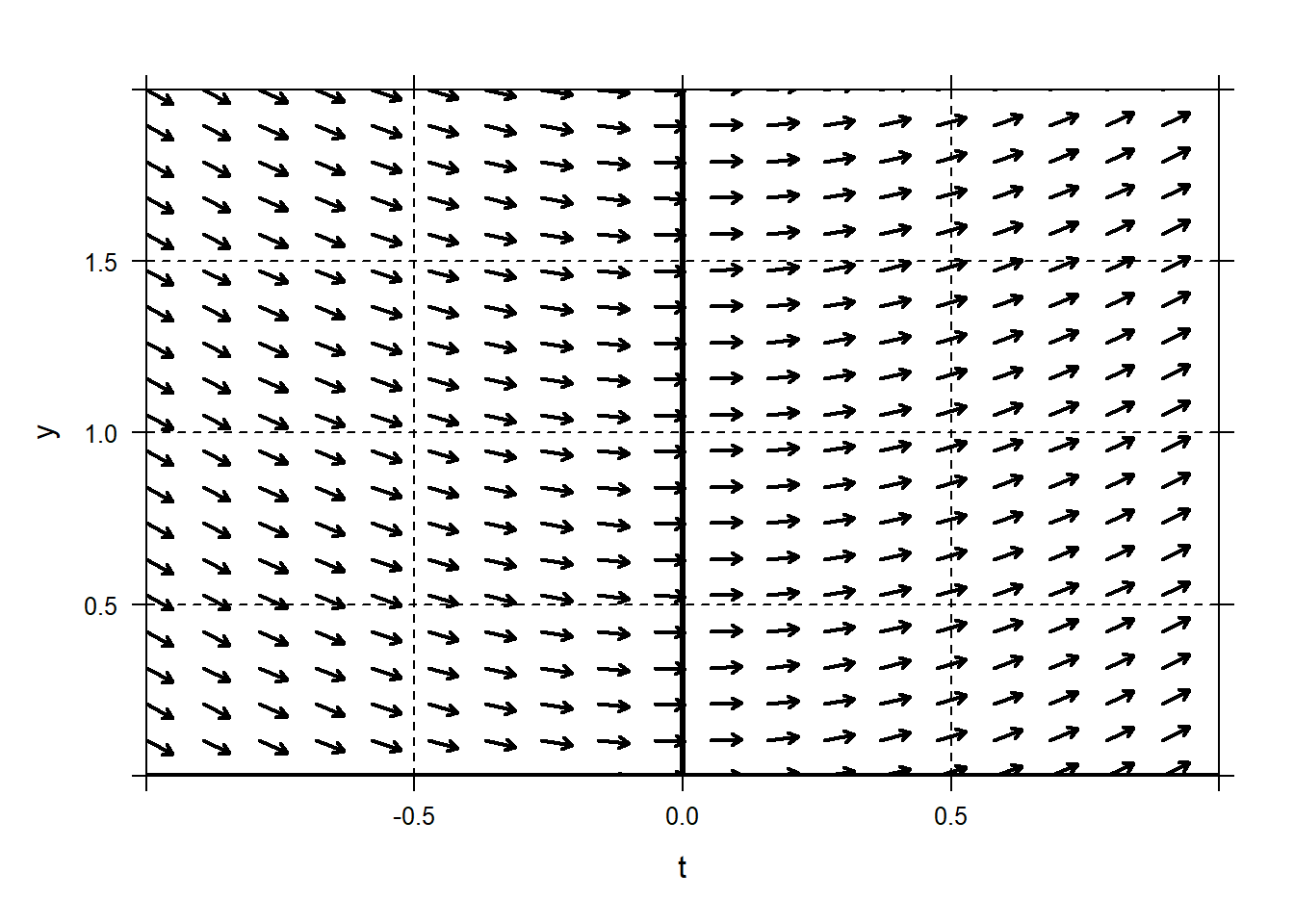
```
plotODEDirectionField(sin(t)~t&y,tlim=c(-1,1),ylim=c(0,2))
mathaxis.on()
grid.on()
```
We know from the initial condtion that the specific solution we are after passes through the point $(t=0,y=1)$. Place a dot at that point to illustrate.
```
plotODEDirectionField(sin(t)~t&y,tlim=c(-1,1),ylim=c(0,2))
mathaxis.on()
grid.on()
plotPoints(1~0,pch='.',cex=10,col="red",add=TRUE)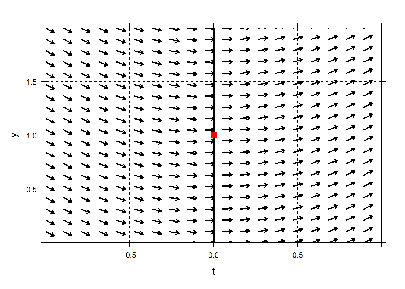
```
We know that if the solution passes through $(t=0,y=1)$ then it must pass parallel to the vectors in the direction field, whose slopes are computed with the ODE. The slope of the tangent line to our solution must be

\[y'=\sin(0)=0.\] Draw a line with slope 0 through the point $(t=0,y=1)$.
```
plotODEDirectionField(sin(t)~t&y,tlim=c(-1,1),ylim=c(0,2))
mathaxis.on()
plotPoints(1~0,pch='.',cex=10,col="red",add=TRUE)    
plotFun(0*x+1~x,lwd=3,col="dodgerblue4",lty=2,add=TRUE)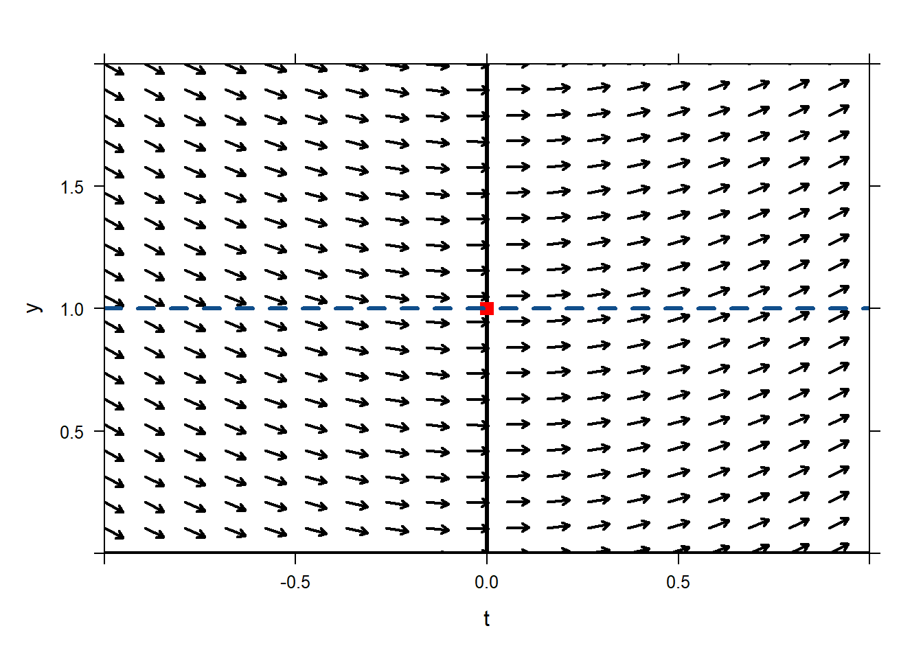
```
We expect our solution to stay close to that line, since it is the tangent line to our solution, at least for a little while. Where is this tangent line at time $0.25$? Using the equation for the tangent line (it has slope 0 and passes through (0,1)) we find that we expect it to be at

\[y=0\cdot(0.25-0)+1=1.\] So we think that our solution will pass close to the point $(t=0.25,y=1)$.
```
plotODEDirectionField(sin(t)~t&y,tlim=c(-1,1),ylim=c(0,2))
mathaxis.on()
plotPoints(1~0,pch='.',cex=10,col="red",add=TRUE)    
plotFun(0*x+1~x,lwd=3,col="dodgerblue4",lty=2,add=TRUE)
plotPoints(1~0.25,pch='.',cex=10,col="red",add=TRUE)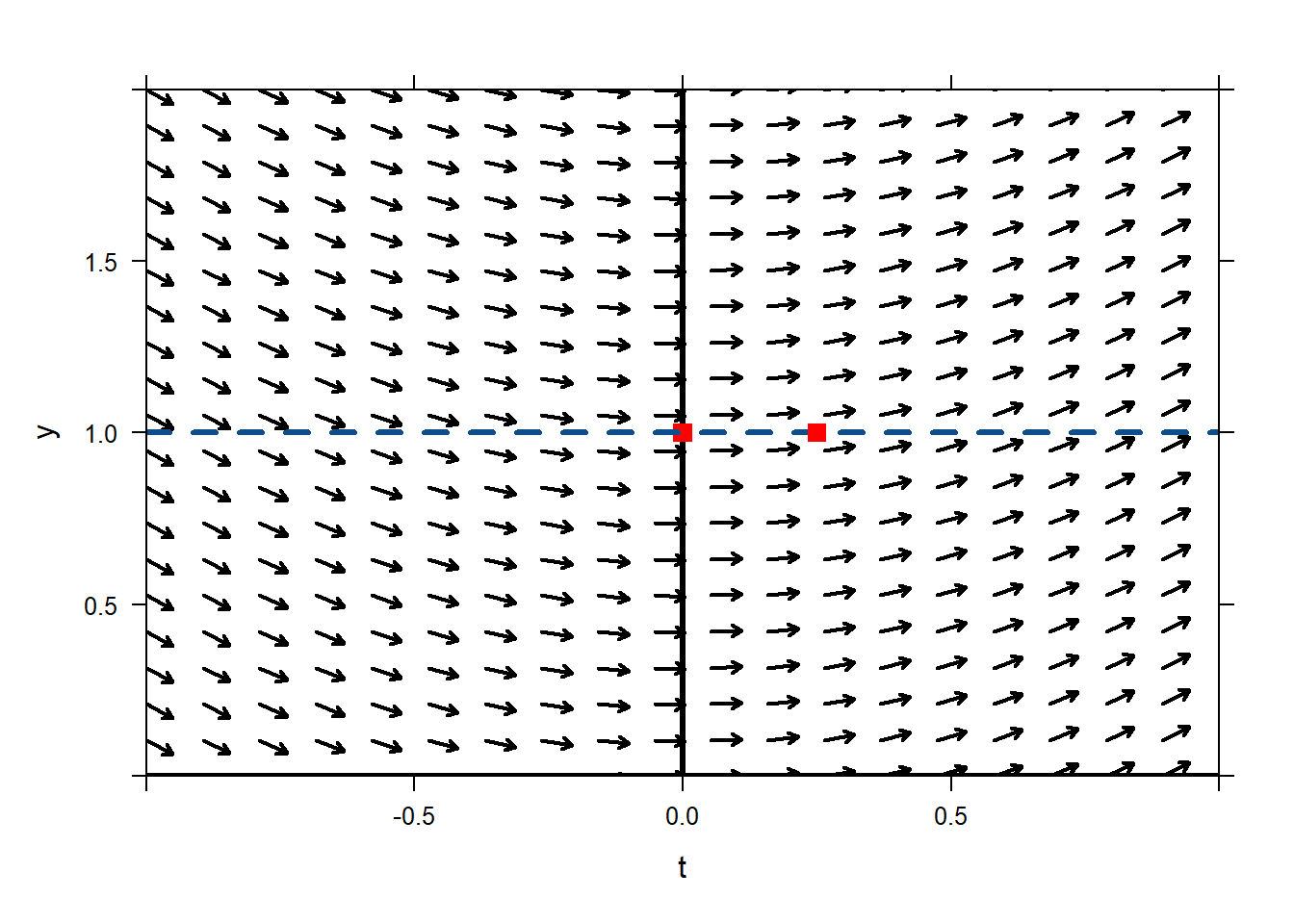
```
In order to keep following the slope field, we’ll redraw a new tangent vector to our solution, assuming that our solution really does pass through $(t=0.25,y=1)$. The slope of the tangent line would be

\[y'=\sin(0.25)=0.247\] Draw the tangent line to our solution; it passes through $(t=0.25,y=1)$ and has slope 0.247.
```
plotODEDirectionField(sin(t)~t&y,tlim=c(-1,1),ylim=c(0,2))
mathaxis.on()
plotPoints(1~0,pch='.',cex=10,col="red",add=TRUE)    
plotFun(0*x+1~x,lwd=3,col="dodgerblue4",lty=2,add=TRUE)
plotPoints(1~0.25,pch='.',cex=10,col="red",add=TRUE)
plotFun(0.247*(x-0.25)+1~x,lwd=3,col="dodgerblue4",lty=2,add=TRUE)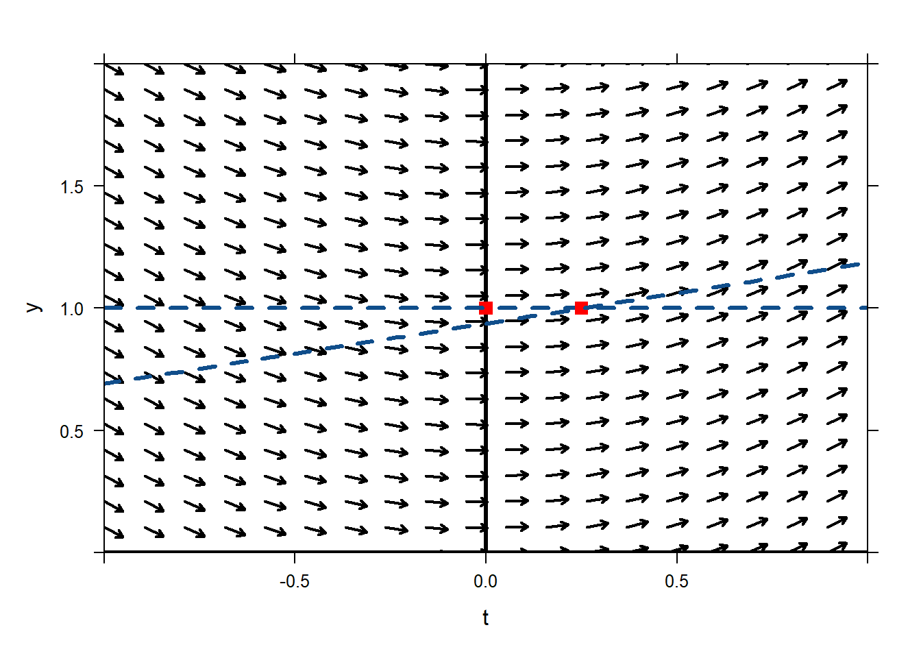
```
Once again, now we have a tangent line to our solution. Where do we expect our solution to get to at time $t=0.5$? If we just use the equation of the tangent line we’ll see that we expect our solution to be at \[y=0.247\cdot(05-0.25)+1= 1.062.\]

So we think our solution will pass close to $(t=0.5,y=1.062)$.
```
plotODEDirectionField(sin(t)~t&y,tlim=c(-1,1),ylim=c(0,2))
mathaxis.on()
plotPoints(1~0,pch='.',cex=10,col="red",add=TRUE)    
plotFun(0*x+1~x,lwd=3,col="dodgerblue4",lty=2,add=TRUE)
plotPoints(1~0.25,pch='.',cex=10,col="red",add=TRUE)
plotFun(0.247*(x-0.25)+1~x,lwd=3,col="dodgerblue4",lty=2,add=TRUE)
plotPoints(1.062~0.50,pch='.',cex=10,col="red",add=TRUE)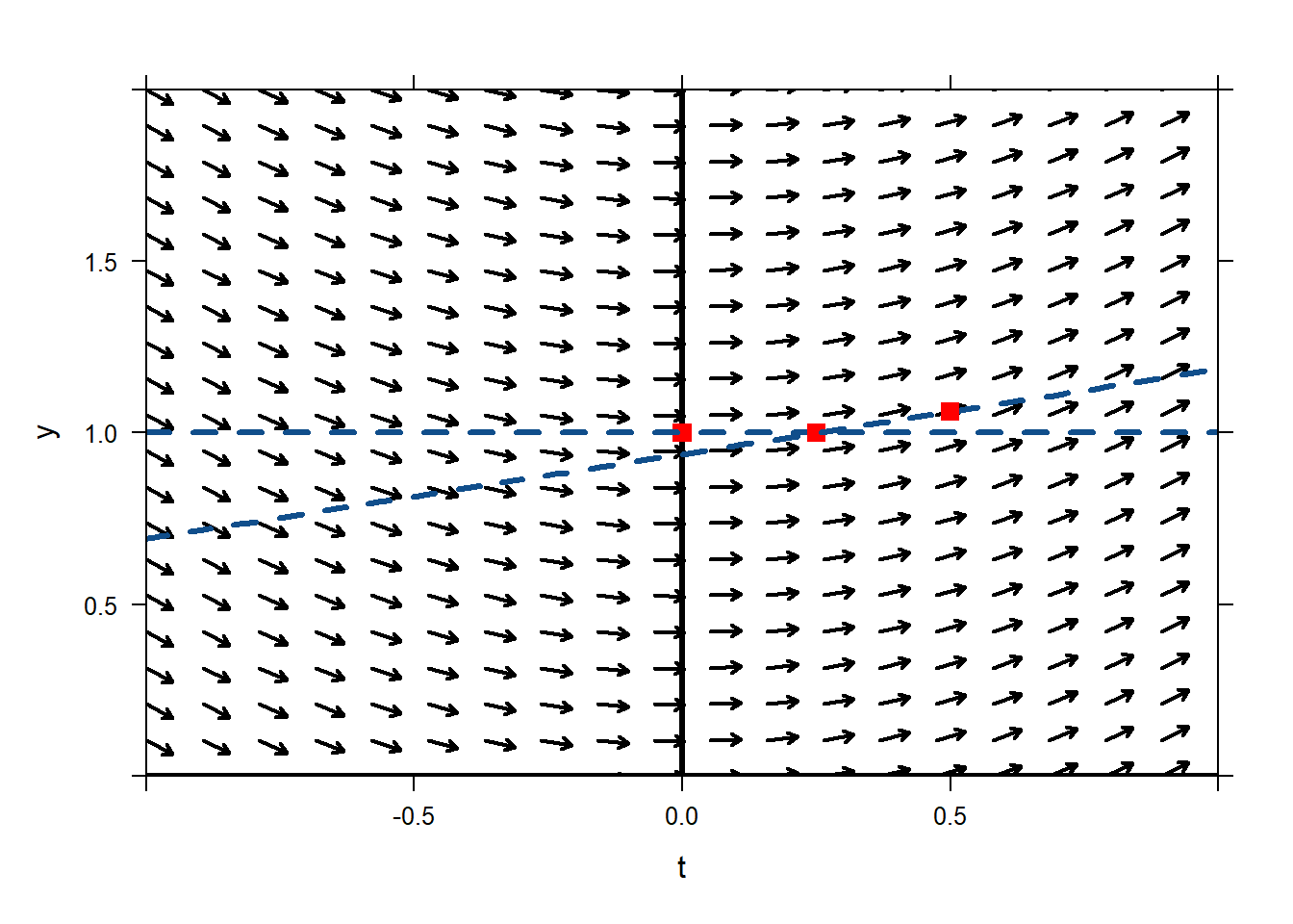
```
One more time for good measure. If our solution passes through $(t=0.5,y=1.062)$ then it must have slope

\[y'=\sin(0.5)=0.479.\]
```
plotODEDirectionField(sin(t)~t&y,tlim=c(-1,1),ylim=c(0,2))
mathaxis.on()
plotPoints(1~0,pch='.',cex=10,col="red",add=TRUE)    
plotFun(0*x+1~x,lwd=3,col="dodgerblue4",lty=2,add=TRUE)
plotPoints(1~0.25,pch='.',cex=10,col="red",add=TRUE)
plotFun(0.247*(x-0.25)+1~x,lwd=3,col="dodgerblue4",lty=2,add=TRUE)
plotPoints(1.062~0.50,pch='.',cex=10,col="red",add=TRUE)
plotFun(0.479*(x-0.5)+1.062~x,lwd=3,col="dodgerblue4",lty=2,add=TRUE)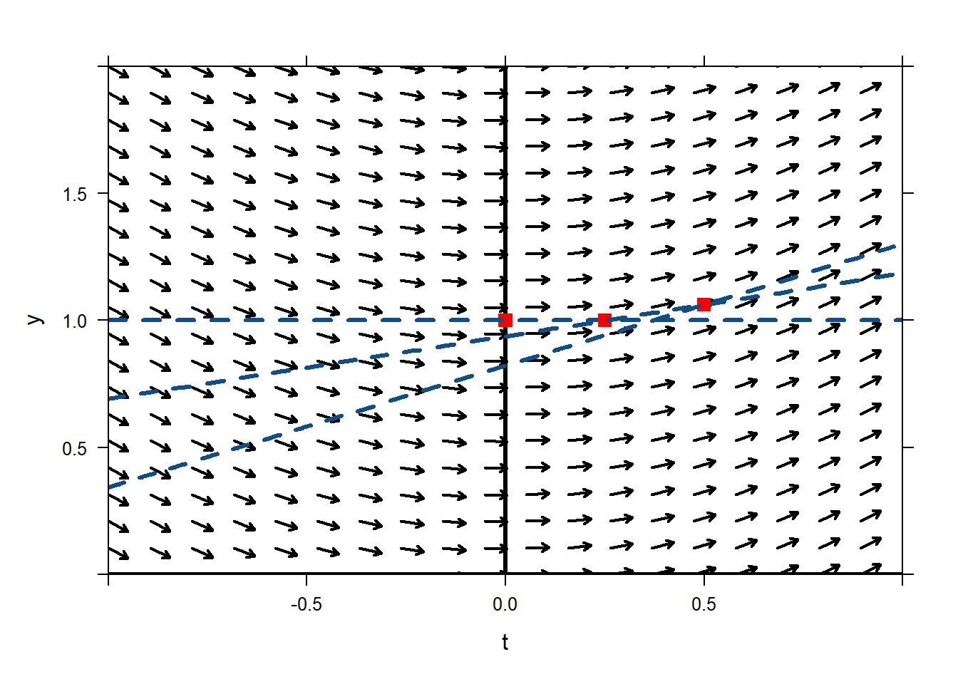
```
We expect our solution to stay close to its tangent line for a little bit. At time $t=0.75$ the tangent line has value \[y=0.479\cdot(0.75-0.5)+1.062=1.182.\] So, we think that our solution must pass approximately through $(0.75,1.182)$.
```
plotODEDirectionField(sin(t)~t&y,tlim=c(-1,1),ylim=c(0,2))
mathaxis.on()
plotPoints(1~0,pch='.',cex=10,col="red",add=TRUE)    
plotFun(0*x+1~x,lwd=3,col="dodgerblue4",lty=2,add=TRUE)
plotPoints(1~0.25,pch='.',cex=10,col="red",add=TRUE)
plotFun(0.247*(x-0.25)+1~x,lwd=3,col="dodgerblue4",lty=2,add=TRUE)
plotPoints(1.062~0.50,pch='.',cex=10,col="red",add=TRUE)
plotFun(0.479*(x-0.5)+1.062~x,lwd=3,col="dodgerblue4",lty=2,add=TRUE)
plotPoints(1.182~0.75,pch='.',cex=10,col="red",add=TRUE)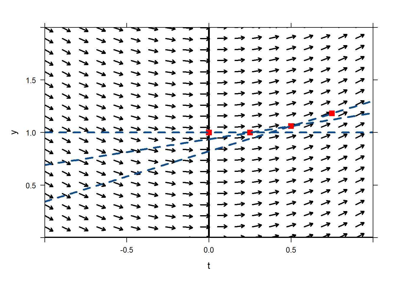
```
Now we can hopefully see a pattern emerging. Again, let $y_n$ be our approximation to $y(t_n)$. We started with the initial condition, so $y_0=y(t_0)=y(0)=1$. We chose our step size to be $\Delta t=0.25$, and estimated the value of $y$ at times $t_1=t_0+0.25=0.25$, $t_2=t_1+0.25=0.5$, $t_3=t_2+0.75$. We calculated \[\begin{aligned} &y(t_1)\approx y_1 = y'_0\cdot \Delta t + y_0 = 1\\ &y(t_2)\approx y_2 = y'_1\cdot \Delta t + y_1 = 1.062\\ &y(t_3)\approx y_3 = y'_2\cdot \Delta t + y_2 = 1.182.\end{aligned}\]

So the pattern seems to be \[y_{n+1}=y'_n\Delta t + y_n,\] where $y'_n$ is calculated from the ODE using the values of $y_n$ and $t_n$.
Either of the above introductions is fine, or you can do something else. At this point, have them compute a few iterations of Euler’s method by hand to compute an approximate solution to \[y'=t-y,\quad y(0)=2\] using step sizes of $\Delta t=0.25$. Have them follow a table like the one in the book to keep things organized. Have them determine how many steps it will take them to approximate the value of the solution at time $t=4$.

Obviously, we do not want to do all the iterations by hand. Besides, computers that approximate solutions for IVPs can use a much smaller step size in order to increase the approximation’s accuracy. Show them how to use Euler to approximate the solution to this problem. You can either only specify the right-hand side:

Euler(t-y~t&y,tlim=c(0,4),stepSize=0.25,ic=2)

##       t         y
## 1  0.00 2.0000000
## 2  0.25 1.5000000
## 3  0.50 1.1875000
## 4  0.75 1.0156250
## 5  1.00 0.9492188
## 6  1.25 0.9619141
## 7  1.50 1.0339355
## 8  1.75 1.1504517
## 9  2.00 1.3003387
## 10 2.25 1.4752541
## 11 2.50 1.6689405
## 12 2.75 1.8767054
## 13 3.00 2.0950291
## 14 3.25 2.3212718
## 15 3.50 2.5534538
## 16 3.75 2.7900904
## 17 4.00 3.0300678

or you can specify the full equation, using _t to denote the derivative.

Euler(y_t=t-y~t&y,tlim=c(0,4),stepSize=0.25,ic=2)

##       t         y
## 1  0.00 2.0000000
## 2  0.25 1.5000000
## 3  0.50 1.1875000
## 4  0.75 1.0156250
## 5  1.00 0.9492188
## 6  1.25 0.9619141
## 7  1.50 1.0339355
## 8  1.75 1.1504517
## 9  2.00 1.3003387
## 10 2.25 1.4752541
## 11 2.50 1.6689405
## 12 2.75 1.8767054
## 13 3.00 2.0950291
## 14 3.25 2.3212718
## 15 3.50 2.5534538
## 16 3.75 2.7900904
## 17 4.00 3.0300678

Euler’s method produces a series of points that approximate the values of the solution to the IVP. Show students how the approximation improves as $\Delta t$ gets smaller. The analytical solution to \[y'=\cos(t),\quad y(0)=0\] is $y=\sin(t)$. Plot the analytical solution as well as the output of Euler’s method for various step sizes.

plotFun(sin(t)~t,tlim=c(0,10),lwd=4,col='darkmagenta')
mathaxis.on()


solution=Euler(cos(t)~t&y,tlim=c(0,10),ic=0,stepSize = 0.5)
plotPoints(y~t,data=solution,col='darkseagreen4',add=TRUE)

solution=Euler(cos(t)~t&y,tlim=c(0,10),ic=0,stepSize = 0.1)
plotPoints(y~t,data=solution,col='darkred',add=TRUE)

solution=Euler(cos(t)~t&y,tlim=c(0,10),ic=0,stepSize = 0.05)
plotPoints(y~t,data=solution,col='deepskyblue4',add=TRUE)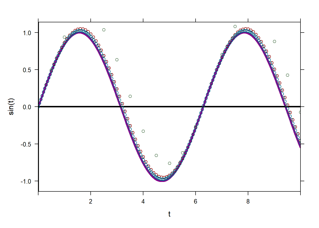

Use the example above to calculate the error in Euler’s method. The error at time step $n$ is defined to be $|y(t_n)-y_n|$. Consider the error in Euler’s method at time 9. Using step size 0.25, time 9 is $t_{36}$.

The value of the analytical solution at time 9 is 0.4121185. The Euler approximation to $y(9)$ is $y_{36}=0.6488611$. The error in Euler’s method at time 9 using step size 0.25 is \[|0.4121185-0.6488611|=0.2367426.\]
```
  tail(Euler(cos(t)~t&y,tlim=c(0,9),ic=0,stepSize=0.25))
```
```
##       t         y
## 32 7.75 1.1014389
## 33 8.00 1.1273875
## 34 8.25 1.0910125
## 35 8.50 0.9945755
## 36 8.75 0.8440725
## 37 9.00 0.6488611
```
```
  abs(sin(9)-0.6488611)
```
```
## [1] 0.2367426
```
If we reduce the step size to 0.1, then the Euler approximation we are after is $y_{90}$. The value of $y_{90}$ is $y_{90}=0.5073315$. The error in Euler’s method at time 9 using step size 0.1 is \[|\sin(9)-y_{90}|=|0.4121185 - 0.5073315|=0.095213\]
```
tail(Euler(cos(t)~t&y,tlim=c(0,9),ic=0,stepSize=0.01))
```
```
##        t         y
## 896 8.95 0.4665841
## 897 8.96 0.4576902
## 898 8.97 0.4487510
## 899 8.98 0.4397674
## 900 8.99 0.4307403
## 901 9.00 0.4216707
```
```
abs(sin(9)-0.5073315)
```
```
## [1] 0.09521301
```
Remember, if we actually had access to the analytical solution of an IVP, then we wouldn’t need Euler’s method. This calculation is for demonstration purposes only. In real life, you never have an exact formula for how much error there is in your Euler approximation.
Repeat this process with an IVP that cannot be solved analytically. Perhaps \[y^{'} = y\sin(t + \sqrt{t})$ \text{ with } $y(0) = 1\].