2.5 Análisis de datos históricos de eventos adversos.

2.5.1 Cargar datos

uu <- "https://raw.githubusercontent.com/vmoprojs/DataLectures/refs/heads/master/Scoring/eventosHistoricos.csv"

datos <- read.csv(uu, sep = ";", dec = ".")
datos$fechaEvento <- sub("sept", "sep", datos$fechaEvento)
datos$fechaEvento <- as.Date(datos$fechaEvento, format = "%d-%b-%y")

2.5.2 Exploración inicial

str(datos)

## 'data.frame':    1117 obs. of  9 variables:
##  $ unidadEjecutora  : chr  "Unidad de Finanzas y Contabilidad" "Unidad de Operaciones  -Préstamos" "Unidad de Administración y Recursos Humanos" "Unidad de Negocios Costa Rica" ...
##  $ fechaEvento      : Date, format: "2018-06-14" "2016-09-07" "2015-10-20" NA ...
##  $ perdidaBruta     : num  247 390 296 195 243 ...
##  $ recuperacion     : num  0 0 0 0 0 0 0 0 0 0 ...
##  $ perdidaReconocida: num  247 390 296 195 243 ...
##  $ detalleNivel3    : chr  "7.1.3 - Incumplimiento de plazos o de responsabilidades" "2.1.1 - Hurto/ robo" "1.2.5 - Falsificación" "7.5.1 - Fallos de contrapartes distintas de clientes" ...
##  $ detalleNivel2    : chr  "7.1 - Recepción, ejecución y mantenimiento de operaciones" "2.1 - Hurto y fraude" "1.2 - Hurto y fraude" "7.5 - Contrapartes comerciales" ...
##  $ detalleNivel1    : chr  "7 - Ejecución, entrega y gestión de procesos" "2 - Fraude externo" "1 - Fraude interno" "7 - Ejecución, entrega y gestión de procesos" ...
##  $ causa            : chr  "Personas" "Eventos externos" "Personas" "Personas" ...

summary(datos)

##  unidadEjecutora     fechaEvento          perdidaBruta       recuperacion     perdidaReconocida  detalleNivel3      detalleNivel2      detalleNivel1     
##  Length:1117        Min.   :2015-03-09   Min.   :  -21.57   Min.   :  0.000   Min.   :  -21.57   Length:1117        Length:1117        Length:1117       
##  Class :character   1st Qu.:2016-05-09   1st Qu.:  116.70   1st Qu.:  0.000   1st Qu.:  119.74   Class :character   Class :character   Class :character  
##  Mode  :character   Median :2017-07-04   Median :  239.08   Median :  0.000   Median :  242.52   Mode  :character   Mode  :character   Mode  :character  
##                     Mean   :2017-07-31   Mean   :  405.68   Mean   :  8.846   Mean   :  414.06                                                           
##                     3rd Qu.:2018-10-21   3rd Qu.:  478.17   3rd Qu.:  0.000   3rd Qu.:  482.10                                                           
##                     Max.   :2020-03-05   Max.   :10500.00   Max.   :739.070   Max.   :10500.00                                                           
##                     NA's   :390                                                                                                                          
##     causa          
##  Length:1117       
##  Class :character  
##  Mode  :character  
##                    
##                    
##                    
## 

sapply(datos, function(x) sum(is.na(x)))

##   unidadEjecutora       fechaEvento      perdidaBruta      recuperacion perdidaReconocida     detalleNivel3     detalleNivel2     detalleNivel1 
##                 0               390                 0                 0                 0                 0                 0                 0 
##             causa 
##                 0

2.5.3 Visualización general

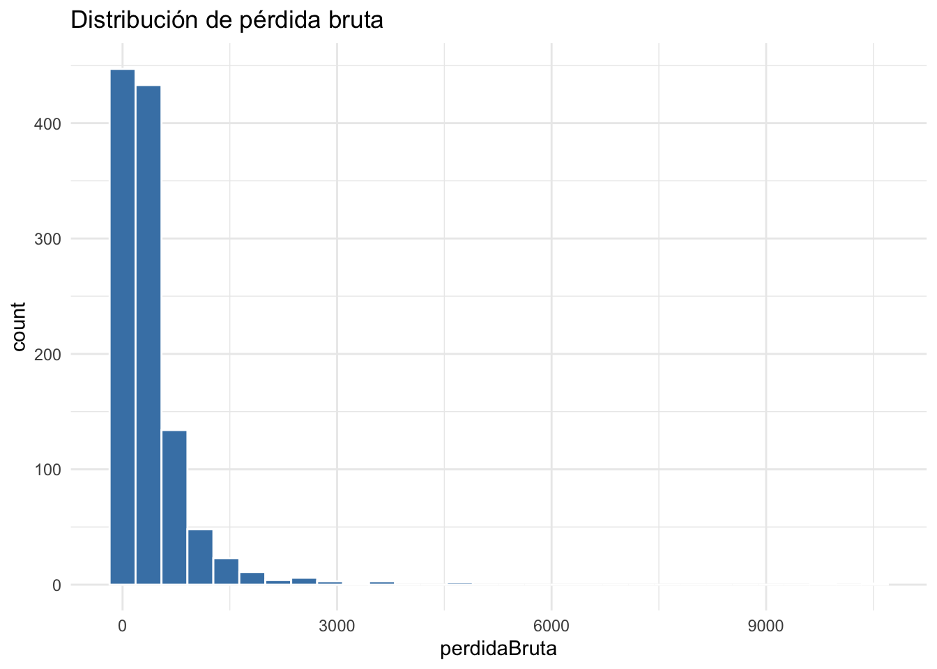
ggplot(datos, aes(x = perdidaBruta)) +
  geom_histogram(bins = 30, fill = "steelblue", color = "white") +
  theme_minimal() +
  labs(title = "Distribución de pérdida bruta")

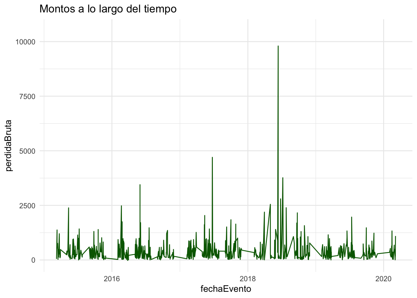
ggplot(datos, aes(x = fechaEvento, y = perdidaBruta)) +
  geom_line(color = "darkgreen") +
  theme_minimal() +
  labs(title = "Montos a lo largo del tiempo")

2.5.4 Pruebas de normalidad

shapiro.test(datos$perdidaBruta)

## 
##  Shapiro-Wilk normality test
## 
## data:  datos$perdidaBruta
## W = 0.4708, p-value < 2.2e-16

2.5.5 Pruebas de hipótesis por causa

# Obtener los niveles únicos
niveles <- unique(datos$causa)
niveles

## [1] "Personas"         "Eventos externos" "Sistemas"

# Función para pruebas por pares
for (i in 1:(length(niveles)-1)) {
  for (j in (i+1):length(niveles)) {
    cat("\n============================\n")
    cat("Comparación:", niveles[i], "vs", niveles[j], "\n")

    grupo1 <- datos$perdidaBruta[datos$causa == niveles[i]]
    grupo2 <- datos$perdidaBruta[datos$causa == niveles[j]]

    # t-test
    cat("\n--- t-test ---\n")
    print(t.test(grupo1, grupo2, var.equal = FALSE))

    # Wilcoxon
    cat("\n--- Wilcoxon test ---\n")
    print(wilcox.test(grupo1, grupo2))

    # Kolmogorov-Smirnov
    cat("\n--- KS test ---\n")
    print(ks.test(grupo1, grupo2))
  }
}

## 
## ============================
## Comparación: Personas vs Eventos externos 
## 
## --- t-test ---
## 
##  Welch Two Sample t-test
## 
## data:  grupo1 and grupo2
## t = 1.34, df = 110.28, p-value = 0.183
## alternative hypothesis: true difference in means is not equal to 0
## 95 percent confidence interval:
##  -32.85096 170.04677
## sample estimates:
## mean of x mean of y 
##  415.8205  347.2226 
## 
## 
## --- Wilcoxon test ---
## 
##  Wilcoxon rank sum test with continuity correction
## 
## data:  grupo1 and grupo2
## W = 46858, p-value = 0.02226
## alternative hypothesis: true location shift is not equal to 0
## 
## 
## --- KS test ---
## 
##  Asymptotic two-sample Kolmogorov-Smirnov test
## 
## data:  grupo1 and grupo2
## D = 0.16085, p-value = 0.03662
## alternative hypothesis: two-sided
## 
## 
## ============================
## Comparación: Personas vs Sistemas 
## 
## --- t-test ---
## 
##  Welch Two Sample t-test
## 
## data:  grupo1 and grupo2
## t = 0.52566, df = 63.564, p-value = 0.601
## alternative hypothesis: true difference in means is not equal to 0
## 95 percent confidence interval:
##  -247.3195  423.9199
## sample estimates:
## mean of x mean of y 
##  415.8205  327.5203 
## 
## 
## --- Wilcoxon test ---
## 
##  Wilcoxon rank sum test with continuity correction
## 
## data:  grupo1 and grupo2
## W = 46063, p-value = 1.399e-11
## alternative hypothesis: true location shift is not equal to 0
## 
## 
## --- KS test ---
## 
##  Asymptotic two-sample Kolmogorov-Smirnov test
## 
## data:  grupo1 and grupo2
## D = 0.44813, p-value = 9.6e-11
## alternative hypothesis: two-sided
## 
## 
## ============================
## Comparación: Eventos externos vs Sistemas 
## 
## --- t-test ---
## 
##  Welch Two Sample t-test
## 
## data:  grupo1 and grupo2
## t = 0.11349, df = 72.16, p-value = 0.91
## alternative hypothesis: true difference in means is not equal to 0
## 95 percent confidence interval:
##  -326.3593  365.7639
## sample estimates:
## mean of x mean of y 
##  347.2226  327.5203 
## 
## 
## --- Wilcoxon test ---
## 
##  Wilcoxon rank sum test with continuity correction
## 
## data:  grupo1 and grupo2
## W = 3700.5, p-value = 3.697e-05
## alternative hypothesis: true location shift is not equal to 0
## 
## 
## --- KS test ---
## 
##  Exact two-sample Kolmogorov-Smirnov test
## 
## data:  grupo1 and grupo2
## D = 0.37302, p-value = 5.98e-05
## alternative hypothesis: two-sided

2.5.6 Correlaciones

cor.test(datos$perdidaBruta, datos$recuperacion, method = "pearson")

## 
##  Pearson's product-moment correlation
## 
## data:  datos$perdidaBruta and datos$recuperacion
## t = 1.9778, df = 1115, p-value = 0.04819
## alternative hypothesis: true correlation is not equal to 0
## 95 percent confidence interval:
##  0.0004741919 0.1173759177
## sample estimates:
##        cor 
## 0.05912777

2.5.7 Boxplot por tipo de evento

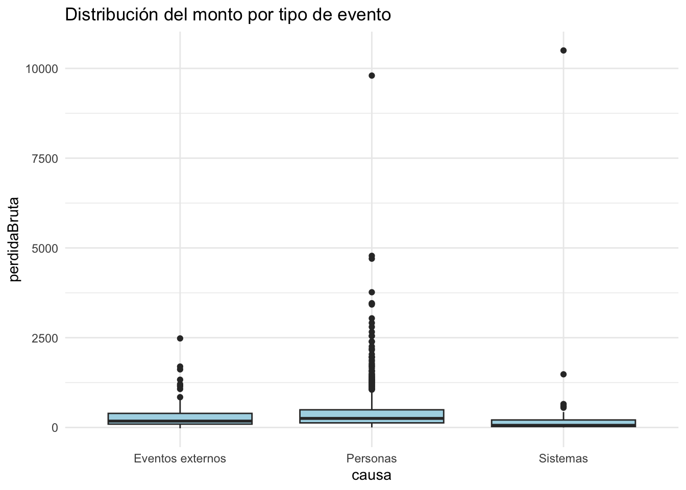
ggplot(datos, aes(x = causa, y = perdidaBruta)) +
  geom_boxplot(fill = "lightblue") +
  theme_minimal() +
  labs(title = "Distribución del monto por tipo de evento")

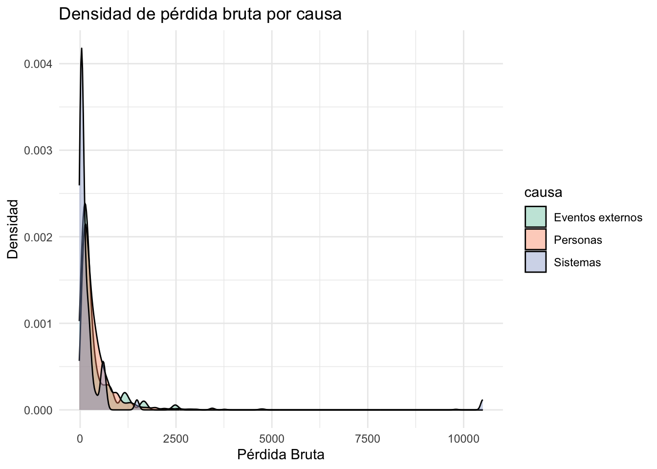
ggplot(datos, aes(x = perdidaBruta, fill = causa)) +
  geom_density(alpha = 0.4) +
  theme_minimal() +
  labs(title = "Densidad de pérdida bruta por causa", x = "Pérdida Bruta", y = "Densidad") +
  scale_fill_brewer(palette = "Set2")