3.5 Assumptions of the General Linear Model
In this chapter I have introduced the General Linear Model informally, as a practical tool with which you can estimate the parameters that you care about. But the General Linear Model makes some assumptions. It’s time to explore what these are, and how you check your data are suitable for applying it. Let’s consider the case of the model m2 that predicts SSRT from Age. Everything I say applies to more complex models like m3 as well, but it is easier to explain it for the case where there is only one predictor.
As mentioned earlier, the model assumes that any value of SSRT, say the value of participant i, is going to be equal to \(\beta_0\), the intercept, plus \(\beta_1\) times the participant’s age.
\[ SSRT_i = \beta_0 + \beta_1 * Age_i \]
This cannot be all, however. If we plot the straight line of SSRT against Age, we see that there is a relationship, but the points do not line up neatly along the line. Have a look (the function abline() adds a regression line with the model specified in its argument):
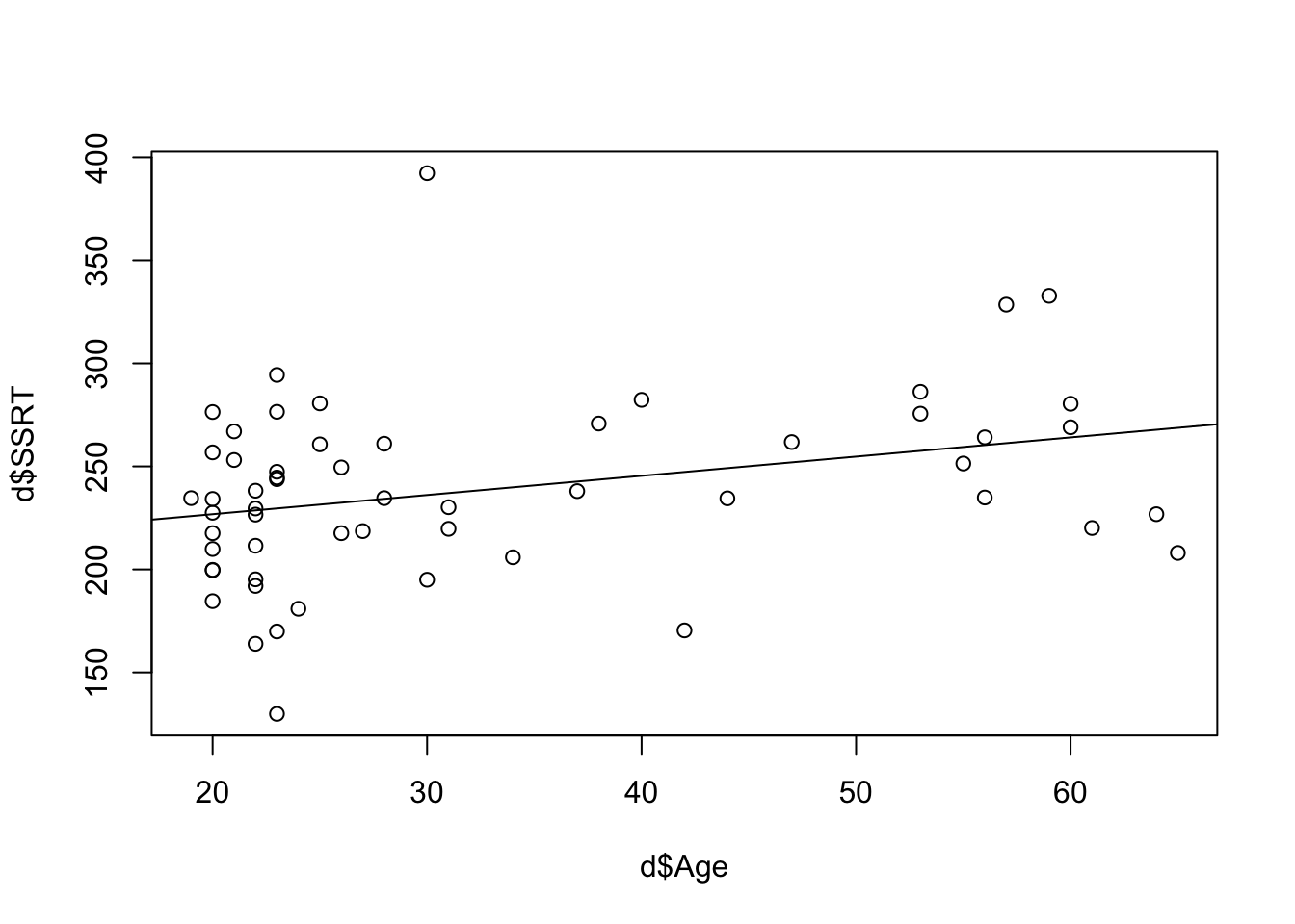
Each point is either above or below the line predicted by just \(\beta_0 + \beta_1 * Age\), by varying distances. The model handles this by assuming there is an error term, a variable representing how far each case is away from the predicted line. The error term reflects that there are many determinants of an SSRT score not included in the predictor variables. We don’t know what the value of the error term is going to be for any particular case of course; that is assumed to be beyond the scope of our knowledge. The model makes two assumptions: one, that the average error is 0 (that is, some points are above and some below the line but there is no systematic direction); and that the errors are generated by processes that lead to a Normal distribution. A Normal distribution is a bell-shaped distribution where most of the errors are small, and larger errors, though possible, are much rarer.
So the full General Linear Model is, formally: \[ \begin{aligned} SSRT_i &= \beta_0 + \beta_1 Age_i + \epsilon_i \\ \epsilon &\sim N(0, \sigma^2) \end{aligned} \]
What does this mean? The first line says: the SSRT of participant i will be \(\beta_0\), plus \(\beta_1\) times their Age, plus some error term \(\epsilon\) whose value is unpredictable from any information included in the model. The second line says: although we don’t know the values of the individual error terms for specific participants, we can assume that they are generated from a Normal distribution with a mean value of 0, and a variance \(\sigma^2\). We don’t know the value of \(\sigma^2\). Just like \(\beta_0\) and \(\beta_1\), the algorithm estimates it using the data.
3.5.1 Checking assumptions: Distributions of residuals
The difference between the fitted value of SSRT for each case (the value given by \(\beta_0 + \beta_1 * Age_i\)) and the actually observed value is known as the residual. The residuals are the empirical manifestation of the errors \(\epsilon\). Because the model assumes that errors are generated from a Normal distribution, the residuals should have a symmetrical, roughly bell-shaped distribution. If this assumption is badly violated, our parameter estimates may be misleading. It is therefore worth checking what the distribution of the residuals looks like. The residuals are stored in a variable that is part of the model object m2. You can look at them with:
 Some residuals are almost 0 (the person’s SSRT is close to the predicted line); others are 50 msec or more, in either the positive or negative direction (the person’s SSRT is higher or lower than predicted). The critical thing is the shape of the distribution of the residuals, so let’s use
 hist() to look at that:
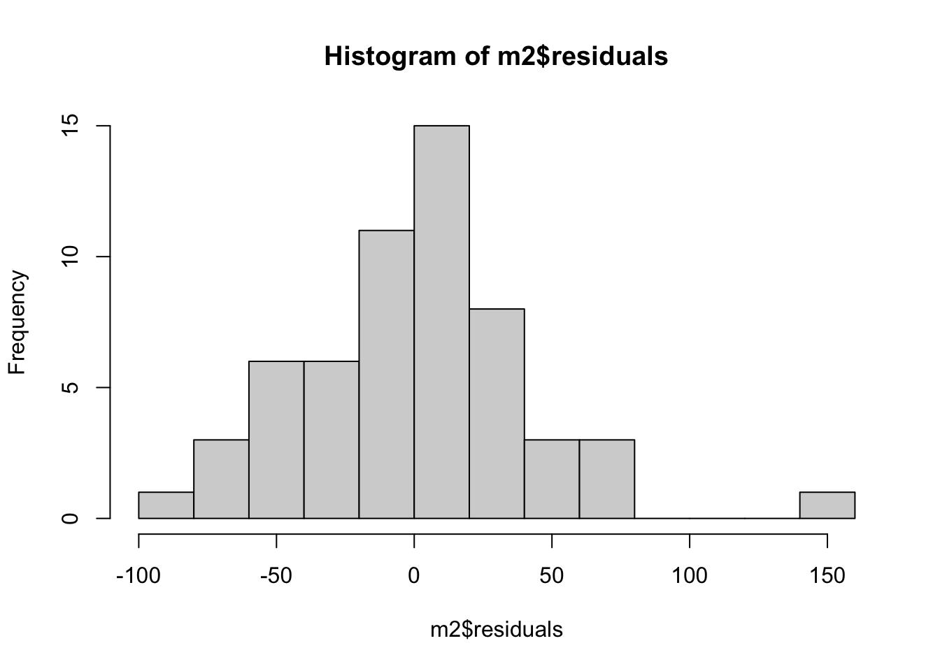
It’s not a disaster, but the distribution is not quite symmetric either. The positive residuals are made up of many very small values and one really big one (about 150 msec) that has no correspondingly large counterpart on the negative side. The question arises: how asymmetric does the distribution of residuals have to be for us to worry about the intepretability of our parameter estimates? It’s a reasonable question but there is not a simple answer.
Some statisics courses teach you to do ‘Normality tests’, statistical tests that are supposed to tell you if your residuals are ‘significantly’ different from those generated by a Normal distribution function. Some statistics courses even tell you to do Normality tests on the outcome variable itself, rather than the residuals!
Normality tests should be avoided, obviously for the outcome variable, but even for the residuals. Why? Because whether a statistical test yields a ‘significant’ result depends to a great extent on the sample size (see section 11.4). If the sample size is small, these tests won’t give you a significant p-value even if the departures from Normality of the residuals are really quite dramatic. If the sample size is very large, the tests will almost always be significant, even if the deviation from Normality is inconsequential. The Normal distribution is a theoretical distribution after all, and no actual dataset corresponds exactly to its distribution function. Even human heights, the classic example of a Normally distributed variable, depart subtly from the theoretical distribution, and so a Normality test would return ‘significant’ if the sample size got large enough.
Instead of a formal test, examine your residual distribution by eye for asymmetry. If you have a marked asymmetry, you may need to transform one or more of your variables (see section 3.5.3).
3.5.2 Checking assumptions: Homogeneity of variance
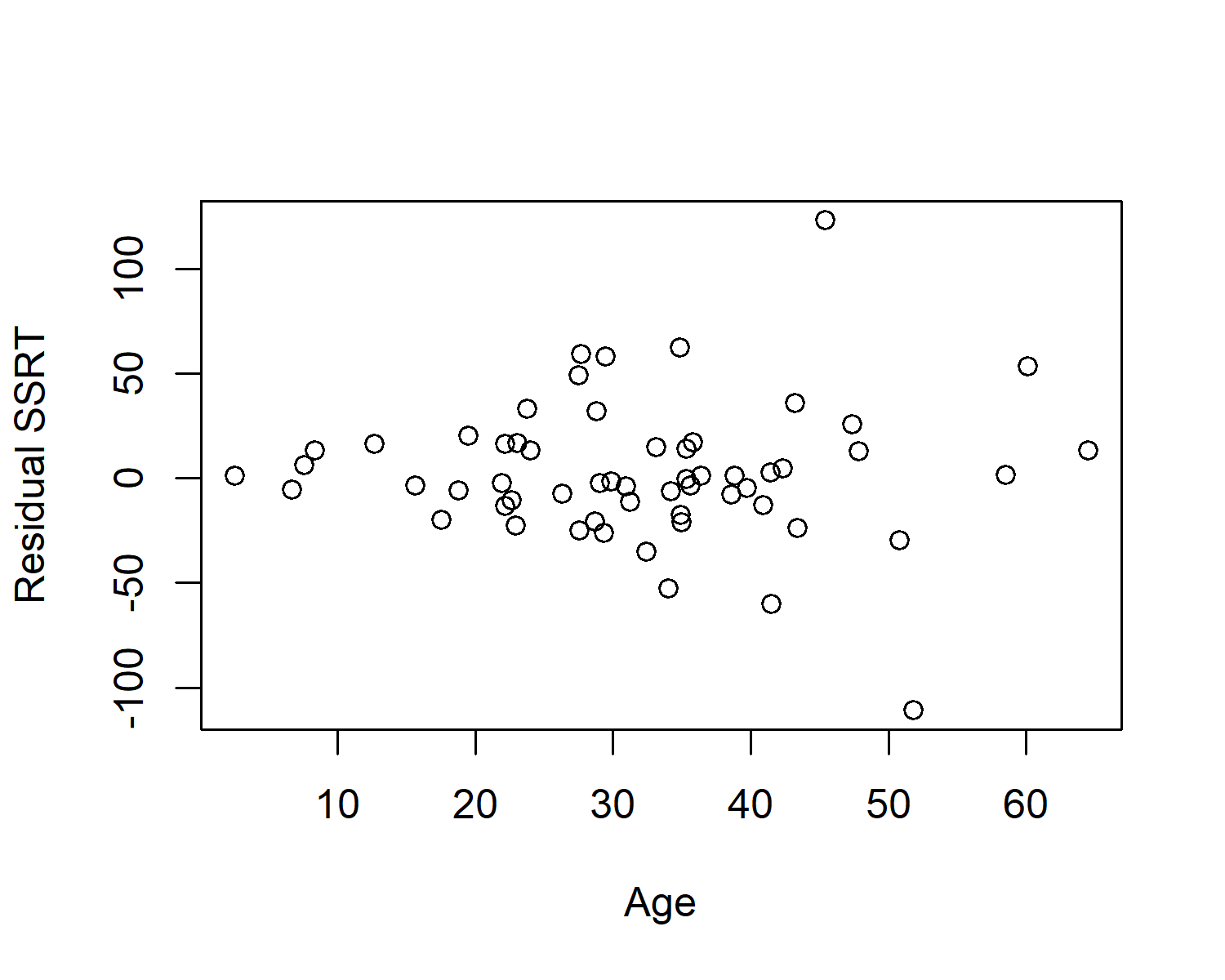
If you look back at the equation for our General Linear Model, the variance of the residuals is a constant, \(\sigma^2\). This means that the dispersion of the residuals should be the same across the whole dataset. It should not change across the range of the predictor variables. The assumption that the variance of the residuals is constant across the range of the predictor variables is known as homogeneity of variance or homoscedasticity. You can assess to what extent your data are compatible with the assumption of homoscedasticity by making a plot of the model residuals against Age. This is slightly fiddly because the Age variable has a missing value. Here is how you do it.
 In the above code,
 is.na() is a function that identifies NA values; !is.na() therefore identifies values that are not NA, because ! in R means ‘not’; and d$Age[!is.na(d$Age)] is the vector of non-missing values of d$Age.
What you are hoping to see is no pattern; the points do not spread out on the vertical dimension as you move from left to right, or indeed as you move from right to left. The dispersion of residuals should be similar at all ages. This one is fine. To give you an example of what you don’t want to see, here’s a hypothetical example where homoscedasticity is violated:
In this hypothetical case, the residuals are tightly clustered around zero in the young people in the sample, but much more variable for the older people in the sample. Violations of homoscedasticity are arguable worse for the reliability of your paramater estimates than violations of Normality in the distribution of residuals.
3.5.3 Transformations
So what are you going to do if the distribution of your residuals is asymmetric or there is an obvious violation of heteroscedasticity? Do not despair. There are solutions. The solution ‘lite’ is to transform one or more of your variables. The solution ‘dramatic’ is to use a different kind of model than a General Linear Model (a Generalized Linear Model or a Generalized Additive Model). We will cover Generalized Linear Models in section 6.2. The rest of the section will look at how to transform your outcome variable for the solution ‘lite’.
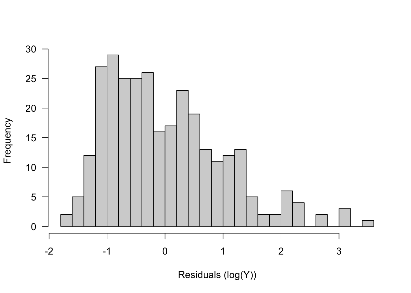
If your problem is that the residuals are positively skewed and/or there is more variation in the residuals at large values of the predictors, then you should consider logarithmic transformation of your outcome. A positively-skewed distribution is one that looks something like this:
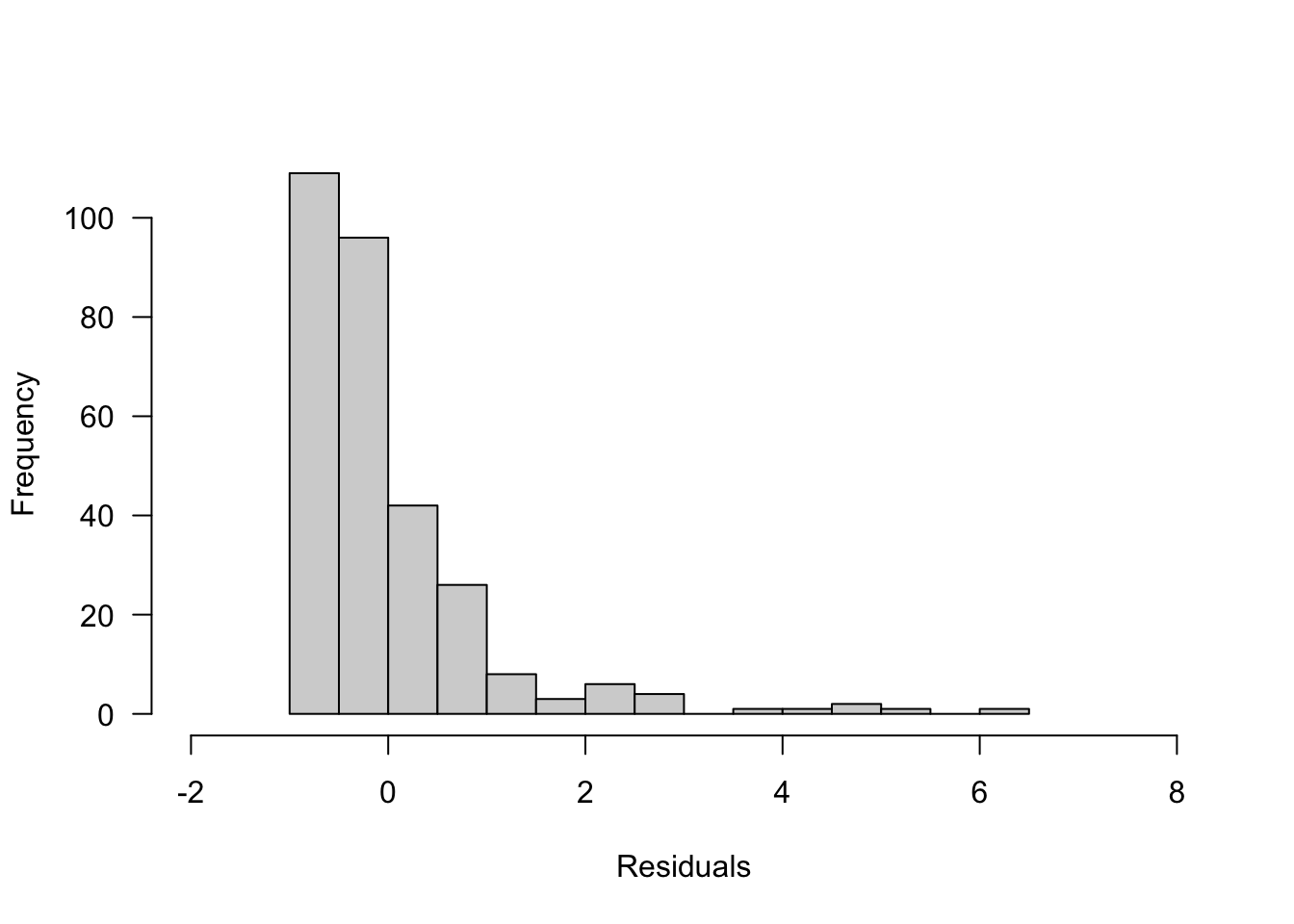
In this case, if you take the logarithm of your outcome variable, the extreme high cases will be ‘pulled in’ towards the centre of the data (because taking the logarithm has a proportionally larger impact on larger values). Your residual distribution will be compressed to the left to look more like this:
You take the (natural) logarithm in R using the function log(). Note that you can only take logarithms of positive numbers, so if your variable contains zeros or negative numbers, you will have to add a constant to every value before logging, to make all values positive.
If your residuals show the opposite pattern, negative skew (long tail to the left) or greater residual variation at low values, you might want to try subtracting the variable values from their maximum value plus 1, to turn the low numbers into high ones, and then logging. Remember though that when you interpret your parameter estimates, high values are now low and vice versa. There are also other transformations (square root, inverse, arcsin) that can be helpful, but I won’t say anything more about them here. Transformation of predictor variables can also be useful if the associations between predictor and outcome are non-linear. In many cases where \(Y\) is non-linearly related to \(X\), you get poor model fit and a strange distribution of residuals with the model \(Y \sim X\), but a better fit with \(Y \sim log(X)\).
Going back to model m2, the homoscedasticity looked ok, but maybe the residuals were somewhat positively skewed. So there would be some justification for running the model using a logarithmic transformation of SSRT instead of the raw values. There are no negative or zero values and so logging will not be a problem. Here is how we do it:
            Estimate Std. Error t value Pr(>|t|)
(Intercept)  5.45838    0.02373  230.03 9.53e-84
Age_centred  0.00394    0.00162    2.43 1.82e-02
This model produces the same conclusion as the untransformed variable. The parameter estimate for Age has a different value, of course, because in m2.logged it represents the change in the logarithm of SSRT with every year’s increase in Age, rather than the change in SSRT itself. If you read the paper carefully, you will see that the researchers considered whether a logarithmic transformation of SSRT might be better, and fitted models this way too. In the end they report the non-logged ones in the paper since, it leads to identical conclusions in this case (as we have just seen). This is not necessarily always the case though: it can make a dramatic difference to what you conclude, especially if the violations are marked.
You should therefore always check carefully for residual normality and violations of homoscedasticity when you use a General Linear Model. If you use a transformation, especially when the case for doing so is not completely clear cut, you should consider reporting the results without the transformation too, for robustness and transparency (see chapter 9).