10.5 Internal meta-analysis
The other situation where meta-analysis can be very useful is within your own series of studies. You will often study the same effect or association in multiple datasets as you proceed, perhaps introducing additional refinements or recruiting multiple sets of participants. In this case, as in the case of reviewing the literature, it is less important to count whether the results were significant or not each time, and more important to synthesize the effect sizes from all the studies to get an overall meta-analytic estimate of the effect. This is called mini-meta-analysis or internal meta-analysis (Goh et al., 2016). Generally, in your own research, the studies will be more similar to one another than in the case of studies drawn from different papers, so it tends to go more smoothly. Not least because you always have access to all the raw data!
You perform internal meta-analysis in exactly the same way as meta-analysis from the literature. I am going to show you this now with a very quick example from a paper we have already met (Nettle & Saxe, 2020). As you may recall, in this paper, the authors were studying the effect of various features of a society on people’s intuitions about the extent to which resources within that society should be redistributed (i.e. shared out equally). One of those features was the society’s cultural heterogeneity, which was manipulated in the first five of the seven studies. Those studies differed in other ways, but they all had a manipulated heterogeneity vs. homogeneity variable, and they all measured basically the same outcome. Thus, we can synthesize the effects of this variable across all five.
The five experiments all featured within-subjects manipulation of heterogeneity vs. homogeneity, and a continuous outcome (ideal redistribution on a scale of 1-100). For a comparable effect size across the five, therefore, I am going to use the parameter estimate (and its standard error) for the heterogeneity IV, from a Linear Mixed Model, using a random effect for participant. I will include the other IVs from each study in the models as covariates, though they are not of interest in the internal meta-analysis.
10.5.1 Preparing the internal meta-analysis
First, we have to go to the paper’s OSF repository (https://osf.io/xrqae/), and identify the file-specific URLs for the first five studies (study1.data.csv,…study5.data.csv). Then we read those in:
d1 <- read_csv('https://osf.io/2fxn7/download')
d2 <- read_csv('https://osf.io/374ed/download')
d3 <- read_csv('https://osf.io/98x26/download')
d4 <- read_csv('https://osf.io/c6kgw/download')
d5 <- read_csv('https://osf.io/5zfje/download')
Let’s make sure that in each data set, we have the heterogeneity variable set up so that the reference category is Homogeneous, and therefore that the parameter estimate will reflect the departure from the reference level when the variable is at the level Heterogeneous.
d1$heterogeneity <- factor(d1$heterogeneity, levels=c("Homogeneous", "Heterogeneous"))
d2$heterogeneity <- factor(d2$heterogeneity, levels=c("Homogeneous", "Heterogeneous"))
d3$heterogeneity <- factor(d3$heterogeneity, levels=c("Homogeneous", "Heterogeneous"))
d4$heterogeneity <- factor(d4$heterogeneity, levels=c("Homogeneous", "Heterogeneous"))
d5$heterogeneity <- factor(d5$heterogeneity, levels=c("Homogeneous", "Heterogeneous"))
Next we fit our mixed models, one for each study. We have additional predictors as well as heterogeneity from each study, depending on that study’s particular design, but let’s always put our predictor of interest first in each model. Note also that I am going to scale the outcome variable, so the parameter estimates are in terms of standard deviations of the outcome.
library(lmerTest)

m1 <- lmer(scale(level)~ heterogeneity + luck + (1|participant), data=d1)
m2 <- lmer(scale(level)~ heterogeneity + luck + (1|participant), data=d2)
m3 <- lmer(scale(level)~ heterogeneity + luck + viewpoint + (1|participant), data=d3)
m4 <- lmer(scale(level)~ heterogeneity + luck + war + (1|participant), data=d4)
m5 <- lmer(scale(level)~ heterogeneity + war + (1|participant), data=d5)
Look at the coefficients from the summary for m1.
                           Estimate Std. Error  df t value Pr(>|t|)
(Intercept)                   0.427     0.0837 326    5.10 5.76e-07
heterogeneityHeterogeneous   -0.138     0.0680 497   -2.03 4.27e-02
luckLow                      -0.623     0.0833 497   -7.48 3.29e-13
luckMedium                   -0.450     0.0833 497   -5.40 1.02e-07
The numbers you are going to want are the -0.138 (the estimate) and the 0.068 (its standard error). You could just type these into a new data frame, but that would be silly (and error-prone), since we can pick them directly out of the model summary as follows:
[1] -0.138And:
[1] 0.068So, to make our data frame for the meta-analysis, we pick out the relevant numbers from all the models as follows:
redist.data <- data.frame(
  b = c(summary(m1)$coefficients["heterogeneityHeterogeneous", "Estimate"],
        summary(m2)$coefficients["heterogeneityHeterogeneous", "Estimate"],
        summary(m3)$coefficients["heterogeneityHeterogeneous", "Estimate"],
        summary(m4)$coefficients["heterogeneityHeterogeneous", "Estimate"],
        summary(m5)$coefficients["heterogeneityHeterogeneous", "Estimate"]),
  se = c(summary(m1)$coefficients["heterogeneityHeterogeneous", "Std. Error"],
        summary(m2)$coefficients["heterogeneityHeterogeneous", "Std. Error"],
        summary(m3)$coefficients["heterogeneityHeterogeneous", "Std. Error"],
        summary(m4)$coefficients["heterogeneityHeterogeneous", "Std. Error"],
        summary(m5)$coefficients["heterogeneityHeterogeneous", "Std. Error"])
  )
Have a look at this data frame and make sure you have the right things. If necessary, get the summaries of the individual models to see how the numbers relate.
        b     se
1 -0.1382 0.0680
2 -0.0832 0.0621
3 -0.1432 0.0522
4 -0.1653 0.0588
5 -0.2510 0.0645
10.5.2 Running the internal meta-analysis
Now it is a simple question of fitting the meta-analysis model.
Random-Effects Model (k = 5; tau^2 estimator: REML)

  logLik  deviance       AIC       BIC      AICc
  5.6624  -11.3247   -7.3247   -8.5521    4.6753

tau^2 (estimated amount of total heterogeneity): 0 (SE = 0.0026)
tau (square root of estimated tau^2 value):      0
I^2 (total heterogeneity / total variability):   0.00%
H^2 (total variability / sampling variability):  1.00

Test for Heterogeneity:
Q(df = 4) = 3.6974, p-val = 0.4485

Model Results:

estimate      se     zval    pval    ci.lb    ci.ub
 -0.1546  0.0270  -5.7272  <.0001  -0.2076  -0.1017  ***

---
Signif. codes:  0 '***' 0.001 '**' 0.01 '*' 0.05 '.' 0.1 ' ' 1
Overall, we find that manipulating the apparent cultural heterogeneity of the society reduces preferred redistribution by 0.1546 standard deviations, with a 95% confidence interval -0.2076 to -0.1017. There is no apparent heterogeneity across the studies beyond what would be expected by sampling variability, as indicated by the non-significant Q statistic, and the \(I^2\) estimate of 0. We can also look at the results on a forest plot.
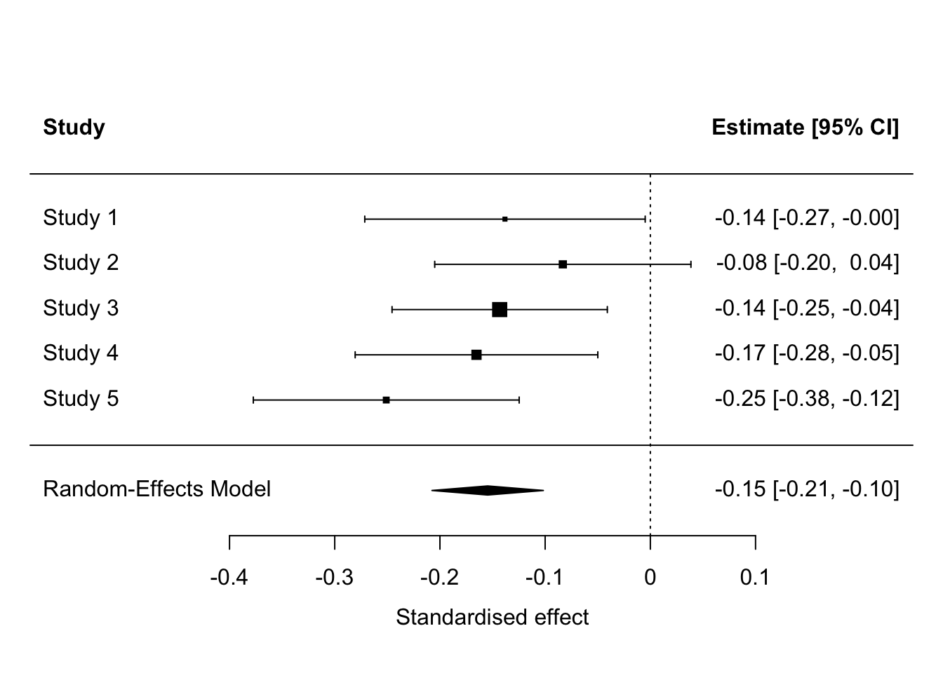
These results are perfectly clear. Although there is some variation in significance in individual studies (the effect in study 2 was not significant), the studies amount to strong support for the existence of a small negative effect of manipulated heterogeneity on preferred redistribution.
10.5.3 What to do with internal meta-analysis
Internal meta-analysis will be useful in many of your projects. These days it is good practice to run a replication study whenever you have an important result (see section 12.2.4). And, you may go on to run variants and refinements within a series of studies, within each of which the same basic comparison is made. You should provide an internal meta-analysis so the reader can see what the evidence adds up to. You can include this in a separate section of the paper, after the reporting of each individual study’s results. Or, you could consider replacing separate Results sections altogether. Analysis of studies separately could go into Supplementary Materials and the main results figure could be something like the forest plot shown above. It really contains all the information the reader needs, in a way that is a lot more concise than five separate Results texts and five separate figures.
A question you might be asking is the following: when should I do an internal meta-analysis, and when should I simply pool the datasets from all the separate studies into one big dataset, and analyse that directly? This is a good question. In the case we have just been through, there were some methodological variations: the studies differed in terms of which other IVs they included, and in a number of other small methodological ways. So here it makes more sense to keep them separate but combine their results through meta-analysis. On the other hand, if your methods across several studies were absolutely identical, or very nearly so, then you can combine all the datasets and do a single analysis of the pooled dataset. In such cases, meta-analysis and pooled analysis should give you broadly the same answer.