11.5 Using power analysis
The previous section used simulation to introduce the main principles of statistical power. This section examines the ways you would use power analysis in your work.
11.5.1 Analytical solutions for power
In the previous section, we used simulated datasets to estimate the power to detect effects of particular sizes at different sample sizes. In fact, it was not necessary for me to do this. For simple cases, there are mathematical formulas that give you the exact power of a test given the sample size and effect size. These formulas are available in the contributed package pwr, for example. So why did I approach power through simulation?
Partly it was a pretext for introducing how to write your own R functions, which is a useful skill. Beyond this, simulating datasets is useful for several reasons other than calculating statistical power. Doing so allows you to try out your analysis strategy and look at what your plots will look like under different assumptions about what you might find. Also, although power formulas exist for simple cases, they do not exist for complex scenarios that you might be trying to get a sense of: data sets with many variables, clustered structure, particular types of covariance between observations or variables. Being good at simulation can provide a tool for getting a sense of what such data sets might look like (or, the range of ways that they could look), and how to analyse them. Finally, I find that approaching power through simulation is a really good way to understand the principles of statistical power thoroughly.
Let’s say that we wanted to directly calculate power for the scenario considered in the previous section. Now is the time to run install.packages('pwr') if you have not done so before. We then use the pwr.t.test() function to calculate our power to detect an effect size of 0.2 standard deviations with a sample size of 50.
     Two-sample t test power calculation

              n = 50
              d = 0.2
      sig.level = 0.05
          power = 0.168
    alternative = two.sided

NOTE: n is number in *each* group
It’s 0.17 or 17%. This should be pretty close to what you got by simulation. In fact we can check the extent to which our simulations gave the same result as the formula. You should have the data frame power.sample.size.data in your environment. If not, regenerate it from the earlier code chunk. We can add an extra column to that data frame, which is the power calculated exactly by pwr.t.test(). Note that we multiply by 100 because the output of pwr.t.test() is a proportion rather than a percentage.
power.sample.size.data$exact <- 100*pwr.t.test(n = power.sample.size.data$Sample.Sizes, d = 0.2)$powerNow let’s add the exact result to our graph as a red line.
ggplot(power.sample.size.data, aes(x=Sample.Sizes, y=Power)) +
  geom_point() +
  geom_line() +
  geom_line(aes(y=exact), colour="red") +
  theme_classic() +
  xlab("Sample size") +
ylab("Power estimated through simulation") 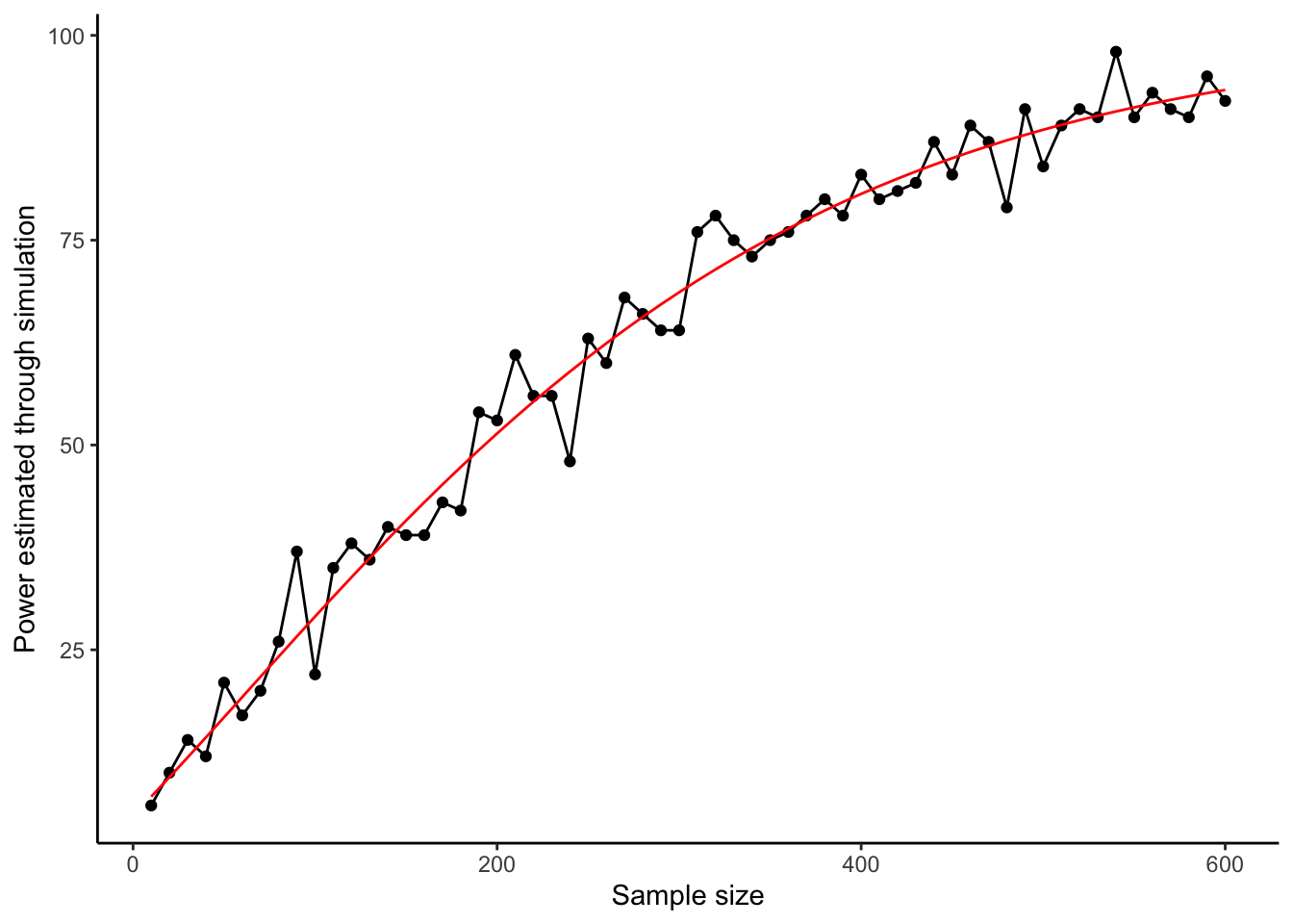
Our simulations did a pretty good job! For an immediate exact result in this simple case, you can go straight to pwr.t.test(). There are other formulas available in the pwr package, each of a different kind of situation and test. It’s worth getting acquainted with which one (if any) is suitable for your needs.
11.5.2 The main ways of using statistical power
Calculation of statistical power is used for the determination and justification of sample size. There are two main ways you might use it (Giner-Sorolla et al., 2024). The difference is whether you: start with an effect size that you want to be able to detect, and then work out what sample size you need to do so with adequate power (sample size determination); or start with a sample size that you have been or will be able to recruit, and then try to figure out what kind of effects you can detect with what power (power determination or minimal detectable effect calculation).
11.5.3 Sample size determination
Sample size determination analysis is the case where you don’t know your target sample size yet. You want to know what it ought to be. Having worked out your study design, you then need to specify a SESOI (smallest effect size of interest, see section 4.3). You put this into the power formulas, or a simulation, and ask: what size sample do I need to have a high chance of detecting the SESOI if it exists? The key issue for this kind of power analysis is choosing the SESOI wisely.
For example, let’s say you want to study the effects of ibuprofen on depressive symptoms. You could ask yourself: how much of an improvement would ibuprofen need to cause in order for it to be a useful part of medical treatment? Presumably if it improved symptoms by 0.01 standard deviations over three months (or something), this would not be very useful in treatment, even if technically not equal to zero. Perhaps we know that placebo pills, for example cause a symptom decrease of a certain magnitude. So the effect of ibuprofen might have to, say, 50% bigger than this before you would rate it as a useful discovery. You would set your SESOI accordingly.
Often you do not have a clear principle like clinical utility to guide you in setting the SESOI. If your study is a replication, you can look at the effect size observed in the study you are replicating. Sometimes there are still findings in the previous literature that help you benchmark the SESOI. For example, you might say ‘I know from previous literature that social isolation causes a 0.4 standard deviation increase in my outcome variable. I think my new manipulation of interest \(X\) is only important if causes an increase of at least this magnitude. If there is an effect, but it is smaller, then \(X\) is not important enough to pursue further. So I will power my study to be able to detect a SESOI of 0.4.’ .
If you really have nothing to go on, you could use the arbitrary conventional values that are often employed: 0.2 standard deviations constitutes a small effect; 0.5 standard deviations a medium effect; and 0.8 standard deviations a large effect. To give you a sense of what each of these means, consider the graphs below of how, in a simple experiment with two groups, the outcome values in the control and experimental conditions will overlap given small, medium and large effects.
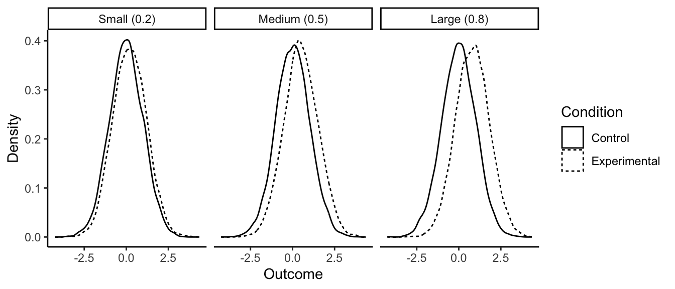
With a small effect (0.2), the means are slightly different, but frankly you need a microscope to see it. The distributions are still almost completely overlapping. Many values from the control condition are higher than many values from the experimental condition, and you certainly can say nothing about which condition a data point came from by looking at the outcome value. With a large effect (0.8), the difference in means is much more obvious. If you guessed which condition a given data point came from based on its value, you would be right much more often than not. But still, even with an effect size of 0.8 standard deviations, the distributions are very overlapping. Your manipulation is certainly not a magic bullet, dwarfing other influences on the outcome.
In experimental studies (especially if you use between-subjects manipulation), if you power for a SESOI of 0.2 you will be running hundreds or even thousands of participants. You have to ask yourself if this is a good use of resources; if the effect is that small, is it really meaningful anyway? If you are testing a theoretical claim, I would be more tempted to reason as follows: my theory does not just say that \(X\) affects \(Y\); it says that \(X\) is an important driver of \(Y\). So if the theory is right, changing \(X\) ought to change \(Y\) by at least a medium effect size. Any less than this and the theory has failed. So, a fair test of the theory is to set my sample size to give me very good power to detect a medium effect size (0.5). If I then don’t see a significant effect, then either: \(X\) has no effect on \(Y\), and the theory has failed; or \(X\) has only a very small effect on \(Y\), and the theory has failed; or I’ve been really unlucky.
However, there are times when even a very small effect of \(X\) on \(Y\), or association between \(X\) and \(Y\), would be theoretically or practically interesting. In such a case, if you have the resources, you should set your sample size up to have good power to detect even a small effect size. But - I warn you - unless you have within-subjects manipulation, this can mean some very large samples.
One question I have glossed over. When I say ‘set your sample size to give you very good power to detect such-and-such an effect’, what does ‘very good power’ consist of? What is the power level I should insist on? It can’t be 100% because power only approaches 100% as the sample size tends to infinity; you never quite get there. If you set it at 95% (the obvious counterpart to the p = 0.05 criterion for significance), you end up spending a lot on running large samples, due to the marked flattening off of the sample size-power curve at its right-hand end. Many traditional statistics texts recommended 80%. Personally, I prefer 90%. If I am going to go to all the trouble of running a study, I would like to have at least a nine in ten chance of detecting my SESOI if it is actually there!
11.5.4 Power determination or minimal detectable effect calculation
The other major case of power analysis is where your sample size is set anyway, by your budget or time window or technology, or just by the number of individuals that are available in the population you are studying. Here, you can’t just decide on a SESOI and then determine the required sample size accordingly. However, you can still use power analysis. You can say ‘given that my sample size is going to be n, then what level of power will I have to detect an effect of 0.5 standard deviations, or 0.2 standard deviations, or any other size of interest?’. This is called a power determination analysis. Or, alternatively, you can say: ‘given that my sample size is going to be n, what is the smallest effect size that I could detect with 90% power?’. This is called calculating your minimal detectable effect.
Using the functions in the pwr package, you generally proceed by supplying any two values from the set of: the effect size; the sample size; and the power. The functions return the third one. So, in pwr.t.test() if you supply it an effect size and a power, it will return the minimum sample size you require (sample size determination); if you give it an effect size and a sample size, it will give you your power (power determination); and if you give it a sample size and a power, it will give you the smallest effect size you can detect with that power (minimal detectable effect determination).