6.3 Generalized Linear Models: Empirical example
6.3.1 The “tomboy”study
We are going to work with the data from a paper on pre-natal exposure to testosterone and “tomboy” identity in girls (Atkinson et al., 2017). The paper is published in a paywall journal (boo!) but at time of writing there is a free PDF version available at: https://eprints.ncl.ac.uk/231669.
‘Tomboys’ are girls who get identified, usually by their parents, as having boy-typical interests or behaviours. The hypothesis of the study was that exposure to higher levels of testosterone in utero will make a girl more likely to develop boy-typical interests and behaviours, and hence more likely to end up being recognised as a ‘tomboy’. As it happens, there is a proxy variable which is supposed to reflect what level of testosterone you were exposed to in utero. This variable is the ratio of the lengths of the second to fourth finger of the right hand (the 2D:4D ratio). A lower 2D:4D ratio is supposed to indicate exposure to higher levels of testosterone in utero (how credible you find the whole study will depend on how credible you find the 2D:4D ratio as a proxy for in utero testosterone). Thus, the hypothesis of the study is that a continuous variable, right hand 2D:4D ratio, will predict a binary outcome, namely answering ‘Yes, I was called a tomboy when I was a girl’, or ‘No, I was not called a tomboy’. The participants were all adult women by the time of the study.
6.3.2 Getting the data
The data for the study are published online on a repository called Github, and there is a link in the paper. If you click on that link, you will see the data. To take the data off and into R, the URL you need is for the “raw” version, and hence not the exact URL given in the paper. I have made a shortcut URL to the right place, which is given in the code below. We are going to call our data frame t for a change.
Now let’s have a look at what our data frame contains:
 [1] "Participant" "Masculine"   "Feminine"    "SRIRatio"    "Androgynous"
 [6] "RIGHT"       "LeftHand"    "Averagehand" "Identity"    "Kinsey"
[11] "Age"         "Tomboy"      "yesOrNo"     "zAge"        "rightHand"
[16] "lnRight"     "lnLeft"      "test"        "id"          "Ethnicity"
This dataset is a bit of a mess, by the way. The variables are not consistently labelled: LeftHand, which is the left hand 2D:4D ratio, starts with a capital letter, rightHand does not, and the rightHand variable is repeated with a different name RIGHT. There are three different variables that represent the outcome: Tomboy codes 1 for tomboys and 2 for not tomboys; yesOrNo codes tomboys as 1 and not tomboys as 0; and id codes the same information in words. Please don’t do this kind of stuff!
We want the outcome variable coded as 1, was identified as a tomboy, or 0, was not, so we will use the variable yesOrNo. In the paper, the authors apply a log transformation to the predictor, but for interpretive clarity in the example that follows, and because it makes no substantive difference, I am not going to do that here. Our predictor variable is thus rightHand
6.3.3 Checking and a quick plot
Let’s have a quick look at what is in the data.
 0  1
26 20
It looks like we have 20 women who were identified as tomboys, and 26 who were not. If the hypothesis of the study is supported, the tomboys will have lower values of rightHand than the non-tomboys. Let’s have a quick look:
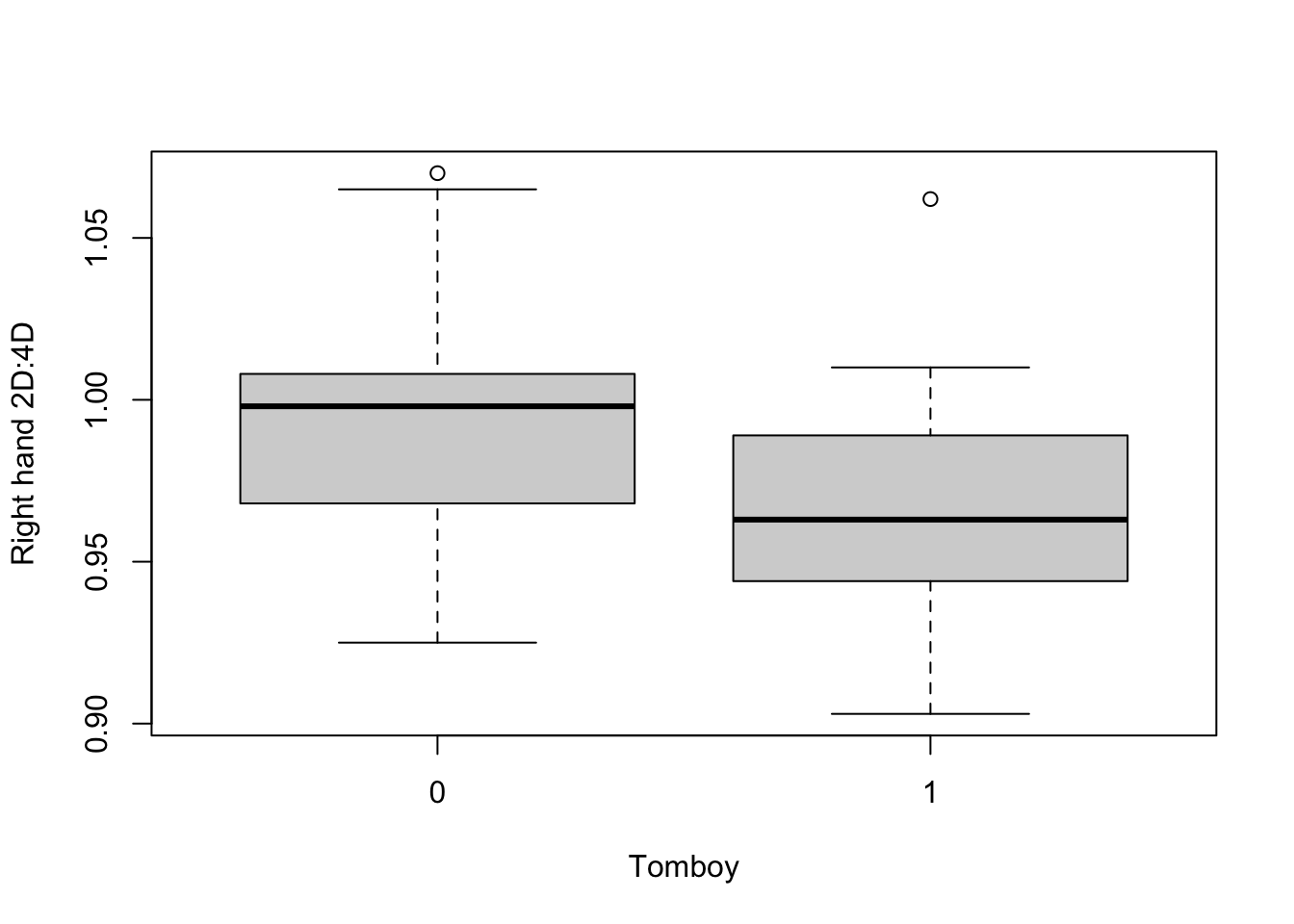
It looks like the hypothesis might be supported. So, it’s time to test this properly with our Generalized Linear Model.
6.3.4 Fitting the Generalized Linear Model
The function we need for our Generalized Linear Model is glm(). The syntax is much the same as the lm() function we have already used, with the additional step that you need to specify the family of your model (here, binomial). We will fit the simplest version of the model at first (i.e. not controlling for any covariates). As before, I am going to centre my continuous predictor variable.
t <- t %>% mutate(rightHand.centred = rightHand - mean(rightHand, na.rm=T))
m1 <- glm(yesOrNo ~ rightHand.centred, family="binomial", data=t)
summary(m1)
Call:
glm(formula = yesOrNo ~ rightHand.centred, family = "binomial",
    data = t)

Coefficients:
                  Estimate Std. Error z value Pr(>|z|)
(Intercept)         -0.322      0.327   -0.99    0.324
rightHand.centred  -19.926      9.432   -2.11    0.035 *
---
Signif. codes:  0 '***' 0.001 '**' 0.01 '*' 0.05 '.' 0.1 ' ' 1

(Dispersion parameter for binomial family taken to be 1)

    Null deviance: 60.176  on 43  degrees of freedom
Residual deviance: 54.790  on 42  degrees of freedom
  (2 observations deleted due to missingness)
AIC: 58.79

Number of Fisher Scoring iterations: 4
We seem to have a significant (p < 0.05) association between the right hand 2D:4D and being a tomboy, with a negative coefficient (-19.93). We can also get the confidence intervals on this parameter estimate:
                    2.5 % 97.5 %
(Intercept)        -0.986  0.309
rightHand.centred -40.583 -2.913
So, the 95% confidence interval for the parameter estimate does not include zero, so we are pretty confident in inferring a negative relationship.
6.3.5 Interpreting the parameter estimate
What does a parameter estimate of -19.93 actually mean? The parameter estimate represents the amount that \(log(\frac{p}{1-p})\) changes for every unit change in rightHand.
To get a sense of how to interpret this, I should first point out that \(\frac{p}{1-p}\) is a quantity called the odds of the outcome. The odds is related to the probability - when the probability of the outcome increases, so does the odds - but they are not the same. For example, an outcome with a probability of 0.9 has odds of \(\frac{0.9}{0.1} = 9\). \(log(\frac{p}{1-p})\) is the logarithm of the odds, and straightforwardly enough, called the log odds. Thus, the parameter estimate for rightHand in model m1 represents the change in log odds of the outcome for every unit change in the predictor. To put that onto the scale of odds, rather than log odds, we use the anti-log function exp():
[1] 2.21e-09The parameter estimate converted in this way represents the odds ratio. The odds ratio is the factor by which the odds by being called a tomboy are changed when right hand 2D:4D increases by one unit.
But wait! The odds ratio here is incredible: 2.211^{-9} is about 0.0000000022. This means that for every unit increase in the right-hand 2D:4D ratio, the odds of being called a tomboy reduces to less than a thousandth of one percent of what it was. How can there possibly be an association that strong?
The problem here is that a one-unit change in the 2D:4D ratio is a ridiculously large change. It is the change involved, for example, of going from having the 2nd and 4th digits the same length (ratio=1), to the 2nd digit being twice as long as the 4th (ratio=2). Industrial accidents aside, there are no people whose 2D:4D ratios differ by this much. So, it is not a very useful parameter estimate in terms of getting a sense of the magnitude of the association.
Instead, this is a case where it would aid interpretation to scale the predictor, so that the parameter estimate represents the change in the log odds of the outcome for every standard deviation increase in rightHand. In the sample, the values of rightHand vary from about 0.9 to about 1.1, and the standard deviation is 0.04. So scaling is going to allow us to work out the odds ratio for being called a tomboy when rightHand changes by 0.04, which is a typical change in the population.
Let’s refit the model (the function scale() both scales and centres):
                 Estimate Std. Error z value Pr(>|z|)
(Intercept)        -0.322      0.327  -0.987   0.3237
scale(rightHand)   -0.793      0.375  -2.113   0.0346
Now you should have a parameter estimate around -0.80 (notice that the significance test is unchanged). Let’s convert this to an odds ratio:
[1] 0.449This makes more sense. The odds ratio of about 0.45 means that when right hand 2D:4D increases by a standard deviation, the odds of being a tomboy are multiplied by a factor of 0.45 (i.e. if they were 1 at baseline, they become 0.45; if they were 2 at baseline, they become 0.90). We can also get the confidence intervals on the odds ratio scale, rather than the log odds scale:
                 2.5 % 97.5 %
(Intercept)      0.373  1.363
scale(rightHand) 0.199  0.891
The 95% confidence interval for the odds ratio goes from around 0.2 to 0.9; not, notably, including 1. One is the odds ratio you get if there is no association; values greater than 1 mean an increase in the predictor increases the odds of the outcome, and values less than 1, as here, mean an increase in the predictor decreases the odds.
In the paper, the authors also investigate adding some covariates such as age and ethnicity to the model. If you wanted to have multiple predictor variables in this way, you just add them to the right-hand side of the equation.
m2 <- glm(yesOrNo ~ scale(rightHand) + Age + Ethnicity,
          family="binomial", data=t)
summary(m2)$coefficients
Estimate Std. Error z value Pr(>|z|)
(Intercept) -0.67930 1.03e+00 -0.65946 0.5096
scale(rightHand) -0.89762 4.03e-01 -2.22712 0.0259
Age -0.00269 2.27e-02 -0.11875 0.9055
Ethnicitychinese -0.73457 1.42e+00 -0.51757 0.6048
Ethnicitymixed -15.40493 2.40e+03 -0.00642 0.9949
Ethnicitywhite 0.73456 9.22e-01 0.79703 0.4254The conclusions are qualitatively unaffected by adding these covariates, and the parameter estimate remains pretty similar.
6.3.6 Other families of Generalized Linear Model
There are many families of Generalized Linear Model, suitable for dealing with outcome variables with different kinds of distribution. You can find information on the other families as and when you need it. Other than the binomial family, the other one that may come up is the Poisson family (Poisson regression). This is a family of models suitable for outcome variables that are counts of things (e.g. how many times did something happen?). Counts have a special distribution because they are bounded at zero (an event cannot happen fewer than 0 times), and can only take integer values. You fit a Poisson family model with glm(y ~x, family="poisson", data=data).