5.5 Models with interactions
This section extends our use of the General Linear Model to the case where there are not just several predictor variables, and you want to allow for statistical interactions. I will explain the idea of an interaction as we go but, in essence, it refers to the possibility that you can’t adequately describe how one predictor variable affects the outcome without referring to the level of another predictor variable. Variables that enter into statistical interaction with another variable of interest are also known as effect modifiers or moderators.
Look at figure2, in the facetted version above, again. It looks like there is a relationship between puritanism_score and coop_score, but the nature of that relationship depends on the level of Condition. In the indulgence condition, it appears to be a negative relationship, whereas in the restraint condition, it appears to be a positive one.
If we think about the design of the study, this makes sense. The puritanism_score variable is a measure of the tendency of the person to hold puritanical attitudes. In the indulgence condition, the participants read that the person in the vignette was indulging in more pleasures. The hypothesis was that they would think he would become less cooperative; and this would be particularly true the more puritanical their attitudes (a stronger negative effect in people higher in puritanism_score). In the restraint condition, they read that he had cut down on pleasures. The hypothesis was that they would think he would become more cooperative, and again, this would be more strongly true the more puritanical their attitudes (so, a stronger positive effect in people higher in puritanism_score). So, the different relationships between puritanism_score and coop_score are expected. The relationship between puritanism_score and coop_score should depend on whether the person is making the judgement in the context of indulgence or restraint; or, equivalently, the effect of Condition will vary in magnitude depending how high in puritanism_score the participant is. This means that you cannot adequately describe the effect of Condition without knowing the value of puritanism_score, or the association with puritanism_score without knowing which Condition we are in.
5.5.1 Start with an additive model
In a situation with a statistical interaction, there are (at least) two predictor variables that matter, and you add a third term, the interaction term that captures within the model the way each predictor modifies the effect of the other. Let’s start with a General Linear Model of the kind we have seen so far. I will first centre puritanism_score:
df7$puritanism_c <- df7$puritanism_score - mean(df7$puritanism_score)
m1 <-lm(coop_score~Condition + puritanism_c, data=df7)
summary(m1)$coefficients
Estimate Std. Error t value Pr(>|t|)
(Intercept) -0.803 0.0598 -13.43 7.63e-34
Conditionrestraint 1.769 0.0861 20.55 1.87e-63
puritanism_c -0.103 0.0474 -2.18 2.99e-02This appears to show that both Condition and puritanism_score matter for coop_score, with a positive coefficient for Condition (higher coop_score in the restraint condition) and a negative coefficient for puritanism_score (lower coop_score the higher the participant’s puritanism_score). However, model m1 is not adequate to the situation. Let’s look at the implied equation of the model:
\[ E(coop\_score) = \beta_0 + \beta_1 * Condition + \beta_2 * puritanism\_score \]
That is, the predicted value of coop_score for a participant is going to be \(\beta_0\), plus \(\beta_1\) if they are in the restraint condition, plus \(\beta_2\) for every unit increase in puritanism_score (remember the \(\beta\) are parameters that the model estimates from the data). In model m1, \(\beta_2\) is the same regardless of condition, which means that we assume that an the impact of an extra unit of puritanism_score is the same in the indulgence condition as in the restraint condition. In model m1, the effects of Condition and puritanism_score on the outcome are just added together. For this reason, m1 is known as an additive model.
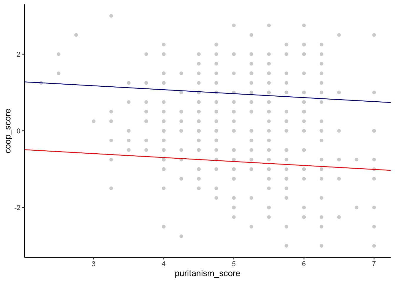
If we wanted to graph what m1 assumes about the situation, it would look as shown below. There is a fit line representing the association between puritanism_score and coop_score for each condition. They can be displaced vertically for the different conditions, because values of coop_score are higher in the restraint condition. But, they are mandated to have the same slope (to be parallel to one another). We know from figure2 that this is not the actual situation.
5.5.2 Specifying and fitting an interaction model
The implied equation of an interaction model looks like this:
\[ \begin{aligned} E(coop\_score)= \beta_0 + \beta_1 * Condition + \beta_2 * puritanism\_score\\ +\beta_3 * Condition*puritanism\_score \end{aligned} \]
Here, the predicted value of someone’s cooperative score would be \(\beta_0\), plus \(\beta_1\) if Condition is restraint, plus \(\beta_2\) for every unit of puritanism_score, plus \(\beta_3\) for every unit of puritanism_score only if the Condition is restraint. Thus, the slope of the relationship between coop_score and puritanism_score is \(\beta_2\) in the indulgence condition, and \(\beta_2 + \beta_3\) in the restraint condition. \(\beta_3\) could end up being estimated at zero, meaning that the slopes are the same in the two conditions. In this case, our interactive model becomes equivalent to m1. But \(\beta_3\) could also end up being estimated at something other than zero, in which case the slopes are different in the two conditions. In this case (whenever \(\beta_3\) is significantly different from zero), we would say that there is an interaction between Condition and puritanism_score.
Let’s fit the interaction model:
m2 <-lm(coop_score ~ Condition + puritanism_c +
          Condition:puritanism_c, data=df7)
summary(m2)$coefficients
We have a significant interaction term (bottom row). The implied slope of
 coop_score on puritanism_score in the indulgence condition is -0.30 (negative, as expected), whereas the implied slope in the restraint condition is \(-0.30 + 0.41 = 0.11\), which is positive, also as expected.
Centring continuous variables is particularly recommended in interaction models, as it makes the parameter estimates easier to interpret. The \(\beta_1\) estimate (1.77) represents the effect of going from indulgence to restraint when puritanism_score is zero. By putting the zero point at the average value of puritanism_score through centring, we have made this an easy quantity to get your head around.
5.5.3 An alternative way of specifying an interaction model
There is also a shorthand way of specifying our interaction model, as follows:
If you fit this you will see that it is identical to m2. So what is the difference? The * notation means ‘these things and all possible interactions between them’. When there are just two predictor variables, this is the same as what we have already done, because there is only one possible interaction between two variables. But, when there are more than two predictor variables, there are many possible interactions (with variables A, B and C, the potential interactions are A:B, A:C, B:C and A:B:C). You might want only some of these in your model as only some are relevant to your hypothesis. Using the full-form specification using the : notation allows you to control which interaction terms should be included in the model, and which ones not.
5.5.4 Interpreting the significance of main effects in models with interactions
In model m2, as well as the interaction term, you have parameter estimates for Conditionrestraint as well as puritanism_score_centred. These estimate parameters \(\beta_1\) and \(\beta_2\). It is tempting to interpret the significance tests associated with these parameters as tests of the hypotheses, respectively, that Condition matters for coop_score, and that puritanism_score matters for coop_score. Be careful! They are not actually tests of those hypotheses. The first one is a test of the hypothesis that Condition matters for coop_score when puritanism_score is zero. The second is a test of whether puritanism_score matters for coop_score when Condition is at its reference category (indulgence). These are more specific hypotheses than whether each variable matters overall, or on average.
If you want to test hypothesis about whether Condition matters for coop_score overall, i.e. regardless of the level of puritanism_score; and whether puritanism_score matters for coop_score averaging across the two Conditions, then you are best off using ANOVA (see chapter 7).