9.2 Running a specification curve analysis

9.2.1 Load in the tomboy data, again

Let us start by reading in the tomboy dataset that we used last time.

library(tidyverse)
t <- read_csv('https://bit.ly/tomboydata')

For specification curve analysis, we are going to use a contributed package called specr, so install it now (install.packages('specr'). Let’s activate it for this session.

library(specr)

9.2.2 Specifying your specifications

To make the specr package do its thing, you need to be able to define some features of the set of possible specifications:

What were all the possible outcome variables (specr calls these y variables; here, only one, yesOrNo);
What were all the possible predictor variables (specr calls these x variables; here, remembering from chapter 6 that in this case it is useful to scale predictors, we have scale(rightHand), scale(log(rightHand)) , scale(LeftHand), scale(log(LeftHand)), scale(AverageHand) and scale(log(AverageHand));
What were all the possible covariates (specr calls these controls; here, Age and Ethnicity);
Were there any subsets of the data we might have used (I don’t think so in this case);
What are all the kinds of models we might want to fit (here, only really the Generalized Linear Model of the binomial family, I don’t think there is any other reasonable choice).

You feed all this information to a function called setup(), which then work out all the possible specifications.

There is one slightly tricky aspect to using specr in this particular case, which is that our Generalized Linear Model of the binomial family is not something it recognises automatically (it handles lm() models without having to do this step). We have therefore to write a user-defined function for fitting this class of model. Don’t worry too much about this bit, it is just to make setup() work with our model, but you do need to run it before you can get any further, trust me.

glm_binomial <- function(formula, data) {
  glm(formula = formula, 
      data = data, 
      family = "binomial")}

Ok, so now we call the setup function:

specs <- setup(data=t, 
               y = "yesOrNo", 
               x = c("scale(lnRight)", 
                     "scale(rightHand)", 
                     "scale(lnLeft)", 
                     "scale(LeftHand)", 
                     "scale(log(Averagehand))", 
                     "scale(Averagehand)"), 
               controls=c("Age", "Ethnicity"), 
               model = "glm_binomial")

As you can see, what we are doing here is listing all the possibilities for the y variable, the x variable, the controls and the kind of model (glm_binomial calls back to the user-defined function we made in the previous chunk of code).

Now we can ask for a summary of our specs object:

summary(specs)

## Setup for the Specification Curve Analysis
## -------------------------------------------
## Class:                      specr.setup -- version: 1.0.0 
## Number of specifications:   24 
## 
## Specifications:
## 
##   Independent variable:     scale(lnRight), scale(rightHand), scale(lnLeft), scale(LeftHand), scale(log(Averagehand)), scale(Averagehand) 
##   Dependent variable:       yesOrNo 
##   Models:                   glm_binomial 
##   Covariates:               no covariates, Age, Ethnicity, Age + Ethnicity 
##   Subsets analyses:         all 
## 
## Function used to extract parameters:
## 
##   function (x) 
## broom::tidy(x, conf.int = TRUE)
## <environment: 0x12167e700>
## 
## 
## Head of specifications table (first 6 rows):

## # A tibble: 6 × 6
##   x                y       model        controls        subsets formula         
##   <chr>            <chr>   <chr>        <chr>           <chr>   <glue>          
## 1 scale(lnRight)   yesOrNo glm_binomial no covariates   all     yesOrNo ~ scale…
## 2 scale(lnRight)   yesOrNo glm_binomial Age             all     yesOrNo ~ scale…
## 3 scale(lnRight)   yesOrNo glm_binomial Ethnicity       all     yesOrNo ~ scale…
## 4 scale(lnRight)   yesOrNo glm_binomial Age + Ethnicity all     yesOrNo ~ scale…
## 5 scale(rightHand) yesOrNo glm_binomial no covariates   all     yesOrNo ~ scale…
## 6 scale(rightHand) yesOrNo glm_binomial Age             all     yesOrNo ~ scale…

We can see that there are 24 specifications, and the first 6 are listed for us.

9.2.3 Running the analysis

Now that we have set up our set of specifications, it is time to run the specification curve analysis, using the function specr(). We do this as follows:

results <- specr(specs)

The best way to examine the output of specr() is to plot results.

plot(results)

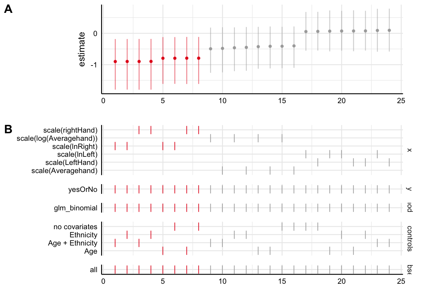
Plot A shows us the parameter estimates for the effect of the x variable on the y variable, for each of the 24 specifications. The ones in red show an association that is significantly different from zero, whilst the ones in grey show those whose confidence intervals overlap zero. As we see, the first eight specifications show our significant negative association, and the next sixteen do not; they show associations around zero.

Plot B shows you what is in each of the specifications in the plot above, showing a tick where a variable is present. So as you can see, the first eight are the specifications that use the right hand 2D:4D rightHand. All of these find the significant associations. In fact, within these eight, it makes remarkably little difference whether we log transform or not, and which covariates we include.

The next sixteen either use Averegehand or leftHand (the inconsistent capitalization for variable names in this dataset makes me foam at the head). As you can see, those that use leftHand produce no hint of a negative association. As you might expect, the parameter estimates for Averegehand are intermediate between those for leftHand and those for rightHand (but, not significantly different from zero). Within the sets using leftHand or Averagehand, again, the decision to log transform or not, or to include covariates or not, makes no perceptible difference.

9.2.4 So what do we conclude in this case?

The conclusion from this specification curve analysis is very clear. The claims made in the paper are totally robust to assumptions about log transforming the predictor variable and the inclusion or exclusion of covariates. Researchers could make any decision in these dimensions and would still come the same conclusion. This is reassuring. On the other hand, the claims are totally dependent on using the right hand for the 2D:4D measurement, not the left hand or the average of the two hands. If the researchers made a different decision here, the conclusion would be no association.

The researchers do acknowledge in the paper that they only find the association using the right hand. Indeed, they cite previous studies also suggesting that it is the right hand that best reflects in utero testosterone, so this makes sense. How you evaluate this is up to you. They did not pre-register that it would be the right hand, not the left, that would predict being a tomboy. And they measured the left hand. And they calculated the average of the two hands as well. So, did they genuinely have an a priori expectation that the right hand 2D:4D but not the left would predict being a tomboy? Or did they try everything and rationalize after the result was known? We can’t tell. This is one of the reasons why preregistration is so good (see section 12.2). It allows us to be clear about which are genuinely prior expectations, and which are just things that make sense after the fact.

In any event, the specification curve analysis neatly shows under what set of specifications you get to the published conclusion, and under what set you do not. This helps us refine our expectations (and plan our analysis strategies) for future confirmatory studies based on these findings.