4.2 Null hypothesis significance tests
The most famous and widespread statistical tests in psychology and behavioural science are null hypothesis significance tests . These are tests of difference, specifically the test that the parameter of interest is different from zero. Let’s start off by getting the behavioural inhibition dataset back, preparing it, and fitting the model we want. If you still have it loaded up from the previous chapter, you don’t need to do anything. If not, run these lines:
# Script to analyse behavioural inhibition data
# Load up tidyverse
library(tidyverse)
# Read in the data
d <- read_csv("https://bit.ly/inhibitiondata")
# Rename the first column
colnames(d)[1] <- "Participant"
# Recode the Condition variable nicer
d <- d %>% mutate(Condition = case_when(Mood_induction_condition == 1 ~ "Negative", Mood_induction_condition == 2 ~ "Neutral"))
# Set the order of the levels of Condition
d$Condition <- factor(d$Condition, levels=c("Neutral", "Negative"))
# Make centered variables
d <- d %>% mutate(
Deprivation_Score_centred =
Deprivation_Score - mean(Deprivation_Score, na.rm=T),
Age_centred = Age - mean(Age, na.rm=T),
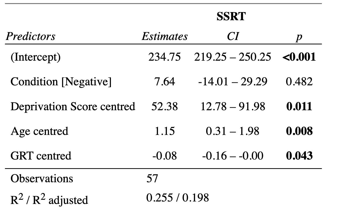
GRT_centred = GRT - mean(GRT, na.rm=T))Once the data is all read, let’s fit model m3 again and get the
coefficients part of the summary.
m3 <- lm(SSRT ~ Condition + Deprivation_Score_centred + Age_centred + GRT_centred, data = d)
summary(m3)$coefficients
Estimate Std. Error t value Pr(>|t|)
(Intercept) 234.7493 7.7250 30.388 8.92e-35
ConditionNegative 7.6383 10.7889 0.708 4.82e-01
Deprivation_Score_centred 52.3777 19.7332 2.654 1.05e-02
Age_centred 1.1483 0.4163 2.759 7.99e-03
GRT_centred -0.0796 0.0383 -2.075 4.30e-02The final two columns in the summary provide a t-value and the
associated p-value (Pr(>|t|)). By the way, R will
often put small or large numbers into scientific notation:
4.297219e-02 is \(4.297219 \,X \,10^{-2}\) or about 0.043. The t-value and p-value are the output you need for a null hypothesis significance test, the test that the parameter in question is equal to zero. The hypothesis that the parameter zero is referred to as a null hypothesis or hypothesis of no effect, since it amounts to the claim that that predictor variable ‘does nothing’ to the outcome variable.
The p-value is directly dictated by the t-value, which in turn is
dictated by the size of the parameter estimate compared to the size of
its standard error. The p-value is an estimate of how likely it is that we would observe a parameter estimate as extreme as the one we did observe in the data, if in fact the parameter in the population was zero. (By ‘as extreme’, we mean ‘at least that far from zero in one direction on the other’). For Age in m3, the probability that we would see a parameter estimate as big as plus or minus 1.15, if in fact the \(\beta\) in the population was zero, is only about 0.008 (i.e. it would happen about 8 times in a thousand).
By convention, if the p-value is less than some criterion value (usually 0.05), then the result is considered statistically significant. In m3, there are
significant null hypothesis significance tests for Deprivation_score, Age and GRT, but not for condition. That’s why there are stars next to the column for those variables (two stars for Age because the p-value is not just less than 0.05, but also less than 0.01 in this case). When the p-value is less than 0.05, we speak of ‘rejecting’ the null hypothesis, and of the result being ‘significant’. On these criteria, we would reject the null hypotheses that Deprivation_score, Age and GRT are unrelated to SSRT (there are significant associations between these variables and the outcome), but accept the null hypothesis that Condition has no effect on SSRT (there is no significant effect).
Imposing the cutoff at p = 0.05 is arbitrary, of course, and imposes a binary (accept or reject) onto what is really a continuum of evidential strength. Note that a null hypothesis significance test is significant with p < 0.05 when and only when the 95% confidence interval for the relevant parameter estimate does not include zero.
4.2.1 What does a significant p-value actually mean?
Tests of null hypotheses using p-values, and the associated idea of ‘significant’ and ‘non-significant’ findings, have become very central to inference in psychology and behavioural science. You will probably use them too. Be careful though: a significant p-value does not mean that the null hypothesis is false; a non-significant one does not mean it is true; and the null hypothesis may not be a sensible one to be testing anyway. The rest of this section reviews some of the reasons these statements are true.
It is worth mentioning why people started to focus so much on null hypotheses. The origins of null hypothesis significance testing come from things like agricultural experiments, in which various substances were put on to crops to see if they made them grow faster. Most of the substances did nothing; they were causally inert and didn’t interact with the physiology of the plant in any way. Those plants grew just like the control plants. A reasonable general prior hypothesis was therefore ‘the treatment will probably do nothing’. What agronomists were looking for is the cases that violated this expectation, the few cases where the substance might do something to the plant. What they wanted was a test procedure that said ‘hang on a minute, this one looks like it might actually do something.’ Starting from the hypothesis of no effect, and having a procedure that shouts ‘this looks significant’ when that hypothesis looks like it might be violated in any way, makes sense for cases like this.
Of course, getting the ‘significant’ result would only be the start. You would then want to ask: are they growing faster or slower, and by how much? These are questions of effect size. It never makes sense to report that a null hypothesis significance test is significant without going on to discuss how big the effect size is, and in which direction.
In many other domains of enquiry, null hypothesis significance testing makes less sense than for agricultural experiments. Imagine you are studying the relationship between the skeletal sizes of different mammals and their body weights. You set up a statistical model in which there is a parameter representing the association between skeleton length and body weight. The idea that this parameter might be zero is not even worth considering. No one could seriously imagine that an elephant with a four-metre skeleton will weigh the same as a rabbit with a 25cm skeleton. It would therefore be crazy to announce the fact that elephants are heavier than rabbits as a ‘significant’ finding (p < 0.05). The epistemic questions in this research are not about whether the parameter is zero (obviously it couldn’t be), but, rather, about the nature of the relationship: is it linear, quadratic, exponential, etc. We will return to the question of when to use null hypothesis significance testing and when not to do so in chapter 8 and section 12.3. Some cases in psychology and behavioural science are like the agricultural experiments, and it works well. Some are more like the elephants and the rabbits, and you should not use it.
4.2.2 False positives
Your p-value can be significant, and yet the null hypothesis can still be true. Such a situation is called a false positive (sometimes also a ‘type 1 error’). Depending on the research topic (specifically, on how likely genuine effects are to occur), most significant p-values may represent false positives (Ioannidis, 2005). How can this be the case?
The fact that false positives can happen stems from the very definition of a p-value. The p-value is the probability that a result at least as extreme as the one you observed could arise by chance if the null hypothesis were actually true. As long as the p-value is not exactly zero, then, the false positive outcome could happen. We know how often we should expect ‘significant’ p-values when the null hypothesis is true: about 5 times for every 100 tests we do (if we are using p < 0.05 as our significance cutoff). The more tests we do, the more false positives we will see (do 20 tests, we will see about one; do 200 tests, we will see about 10).
But how can most significant results represent false positives? Let’s say for example I want to test whether various herbs improve memory function. The vast majority of herbs do not. Most herbs have no systematic effects on the brain (if they did, those effects would probably have been discovered long before now). So, the rate of encountering a genuine new effect of an herb on memory is going to be very low. Let’s be open-minded and say that about 1 in 10,000 herbs we might screen does have a genuine, currently unknown effect. I conduct trial after trial using different herbs. In one of these trials, I get data leading to a significant null hypothesis significance test with a p-value of 0.03. So, there is a 3% chance of getting such a result by chance if the null hypothesis is true and the herb does nothing. On the other hand, the chance that I have actually hit a genuine new effect is, as specified above, 1 in 10,0000 or 0.0001. Now what should we believe? The probability is 0.03 that we would see the outcome we saw by chance, and 0.0001 that we would make a genuine new discovery about the world. Our result is, in other words, something like 300 times more likely to be a false positive than a true discovery, even though the result is ‘significant’.
You can improve this situation quite a bit by reducing the criterion p-value for significance (known as the alpha level) from 0.05 to 0.01 or 0.005. But the point stands in general. At best, a significant p-value says ‘this result looks like it deserves further investigation’. Without replication in another sample, it does not constitute anything like knowledge. There are things you can do other than replication in a new sample to make your significant p-value more credible as the basis for claims: having a good sample size, minimizing the number of statistical tests you do, and always pre-registering your predictions and analysis plan. We deal with these in detail in chapter12.
4.2.3 False negatives
It is bad enough that p-values can often be significant when the null hypothesis is true. They often return ‘not significant’ even when the null hypothesis is false. This is known as a false negative (or type 2 error). The most obvious reason for a false negative is that your sample size is too small. When your sample size is small, the confidence intervals for your parameter estimates must be wide, because you don’t have very much information to estimate parameters well (look back at the figure on how the margin of error of an estimate varies with sample size in section 3.2.2). Very wide confidence intervals may well contain zero even if the parameter estimate itself (the middle of the interval) is some way from zero.
As your sample size gets bigger, the confidence intervals get tighter, statistical tests gain in statistical power (see section 11.4). That is, they become more and more likely to avoid a false negative given that an effect of a certain size really exists. The very same parameter estimate that is ‘non-significant’ with a small sample size will eventually become ‘significant’ as the sample size increases, to the point where in a truly vast sample, the tiniest effect will be ‘significant’. This does not mean of course that the effect matters, either practically or theoretically; only that you have enough precision to distinguish it from zero if the sample is massive.
In sum, which effects are ‘significant’ and which are not is driven very strongly by sample size. If your effect is not significant, this does not mean the null hypothesis is true; only that, with this sample size, you were unable to distinguish it from zero with confidence. Indeed, there is a philosophical question about what it would even mean for the null hypothesis to be true. In the case of SSRT and Age, for example, if average SSRT went up by 0.000000001 msec per year of age, is the null hypothesis true or not? Strictly it is not, since 0.000000001 is not 0; but for all practical purposes it is, since the difference in SSRT between a centenarian and an 18-year old will be much too small to matter in any conceivable way. You could maybe get a parameter estimate of 0.000000001 to be ‘significant’ by testing enough participants (you would need millions), but it is not clear what it would really mean. This reminds us, again, that we always need to be thinking about effect size: not just, is there a relationship between Age and SSRT, but how strong a relationship is it? On that note, what measures of effect size are available to us, and which ones should we use?
4.2.4 Standardised effect sizes
As discussed in the previous sections, alongside any null hypothesis significance test, you want to present what the effect size was (i.e. how big was the difference, or the association?).
Your model summary already gives you measures of effect size: the
coefficients themselves (column Estimates). These show you, in model m3 for example, that being in the Negative rather than Neutral condition was associated with SSRT scores higher by 7.63 msec; and SSRT went up by 1.15 msec with every year of Age.
The problem with these estimates is that they are not only a
transferably intelligible scale. Let’s say there is another study of mood and behavioural inhibition. They found a significant effect of
Condition. But, their behavioural inhibition task was a different one, where participants got a score between 0 and 9 (our SSRT values, by contrast, varied between 130 and 392). In that other study, the effect size for Condition was 0.5. That is a lot smaller than our 7.63. But on the other hand, maybe moving 0.5 points along a scale from 0 to 9 is in some sense a bigger effect than moving 7.63 msec along a scale of 130 to 392 msec. We need to measure these effects on a comparable scale.
Similar problems arise when we compare coefficients for different
predictors within the same study. Look at the summary of m3. The
effect size for Deprivation_score is 53, nearly 50 times stronger than the effect size for Age. But again this difference in magnitude
represents a difference in what one unit change in the predictor
variable means in the two cases. Deprivation_score ranges from 0 to 1, and so a one-unit change is the change from the most deprived place
possible to the least deprived place possible. By contrast, Age is in years, so a one-unit change in age is one year, a rather small change. Deprivation_score is not really more strongly associated with SSRT than Age is: the scales are just very different.
You solve these problems of incomparability of effect sizes by
calculating standardised effect sizes. A standardised effect size is a measure of how many standard deviations of change in the outcome are there when the predictor changes. Standardised effect sizes can be compared across studies or variables that used different scales of measurement. We get standardised effect sizes for our model using the contributed package parameters. Now is the moment to install.packages('parameters') if you have not done so before.
Now try the following:
# Standardization method: refit

Parameter                 | Std. Coef. |         95% CI
-------------------------------------------------------
(Intercept)               |      -0.09 | [-0.44,  0.26]
Condition [Negative]      |       0.17 | [-0.32,  0.66]
Deprivation Score centred |       0.32 | [ 0.08,  0.57]
Age centred               |       0.38 | [ 0.10,  0.66]
GRT centred               |      -0.29 | [-0.57, -0.01]
For the continuous predictors, the Std. Coef represents how many
standard deviations SSRT changes by when the predictor changes by a
standard deviation. This is also known as the standardised regression coefficient, \(\boldsymbol{\text{standardised } \beta}\) or just \(\boldsymbol \beta\). You see that the \(\beta\) for Age is actually a bit bigger than the \(\beta\) for Deprivation_score, when they are put on comparable scales.
For binary predictors like Condition, Std. Coef represents the difference between the two conditions in standard deviations of the outcome variable. This is also known as a Standardised Mean Difference or SMD. Two estimators of the SMD that you might come across are Cohen’s d and Hedges’ g. These differ only by a correction for small sample size, and in large samples they are virtually identical.
The good thing about showing standardised effect sizes is that experienced readers can immediately get a sense of how big effects and associations are, by comparison with their knowledge of past studies they have read. A standardised effect size of 0.2 is pretty small, even if significant (in psychology at least; in sociology and epidemiology, where you are often considering many weak determinants of noisy outcomes in large datasets, this might be considered moderate). A standardised effect size of 0.4 or more starts to be worth considering noteworthy.
4.2.5 Reporting the results of models
When you fit a General Linear Model and consider null hypothesis significance tests of the parameters, you should report the results fully. You should say which terms were included as predictors. For a term of interest, you should not just give the p-value in isolation. Rather, you need to include:
An estimate: either the parameter estimate as it comes out of the model, or a standardised effect size
An indication of precision: Either the standard error, or the 95% confidence interval (not both), for whichever estimate you have given.
The test statistics. This means both the t-value and the p-value.
As an alternative to reporting in text, you might consider showing your model results in tabular form. There are many nice packages for doing this. The function tab_model() in package sjPlot is handy, though it does not show the t-value but only the p-value, thus violating my recommendation above.
In your Viewer window, you should have an output that looks something like this: