10.4 Meta-analysis of the literature
In this example, we are going to imagine we are doing a meta-analysis of studies on whether taking part in mindfulness meditation increases the physiological activity of an enzyme called telomerase. Telomerase is involved in cellular repair; you can think of it informally as reversing the effects of ageing and damage. To cut a complex story short, increasing telomerase activity should generally be associated with better health and slower ageing in the long run. Meditation has been observed to be correlated with better health; these studies are driving to delve into the mechanisms by which such an effect, if it is causal, could come about.
For the sake of the example, we are going to assume we have done a search and found three studies (Daubenmier et al., 2011; Ho et al., 2012; Lavretsky et al., 2013). In reality there are more than three, but these three are sufficient for an illustration. We return to how you would have got to your set of three at the end of the section.
10.4.1 Working out what data to extract
Having established your set of studies, the first thing to do is to read them all and ask yourself the question: is there some statistic they all report that is comparable? Only if you can find such a common currency can you complete your meta-analysis. It’s usually a bit messy since the reporting of different studies is so variable, you have to make some judgements, and sometimes you have to compare the only-roughly-comparable, as you will see here. Sometimes you have one type of effect size estimate (say a correlation coefficient) from some of your studies, and a different type (say an odds ratio) from others. In such a case you will have to use conversion formulas, such as those available through the effectsize package.
Here, all three studies include a control group who did not do mindfulness meditation and a treatment group who did. They all measured telomerase activity before and after the treatment in both groups. Then they do various statistical tests, not necessarily the same ones. However, all report, in their tables, some descriptive statistics of telomerase activity values in each group after the treatment, and we can make use of these. Let’s have a look at the relevant parts of the papers. Here are the relevant tables from the first two:
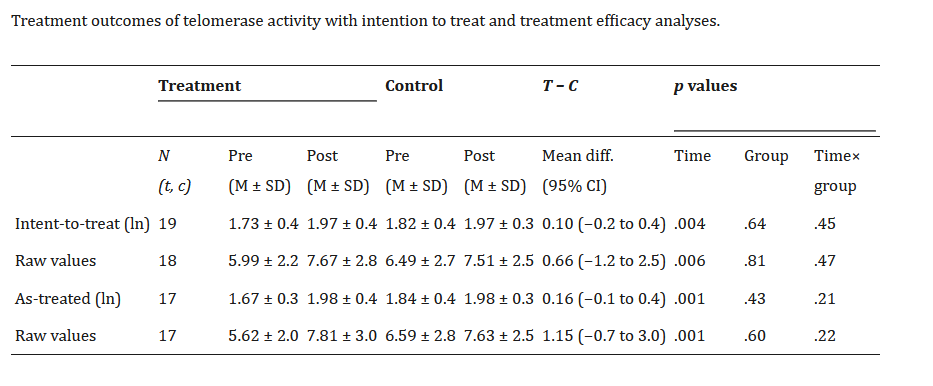
 The table from the first study gives you a choice of raw telomerase values, or log-transformed ones. Since the other studies don’t give the log-transformed ones, we will have to prefer the raw ones. It also defines the groups in two different ways: intention to treat (group membership as originally assigned); and as treated (what the participants actually did). These are not identical since someone was assigned to do the meditation but did not actually do it. We will go with intention to treat; it is not going to make much difference, and it is conservative in terms of estimating the effect size. The table from the second study gives us mean and standard deviation of telomerase activity for the two groups after the intervention. We can make this comparable with the first study.
Now here is the table from the third study:
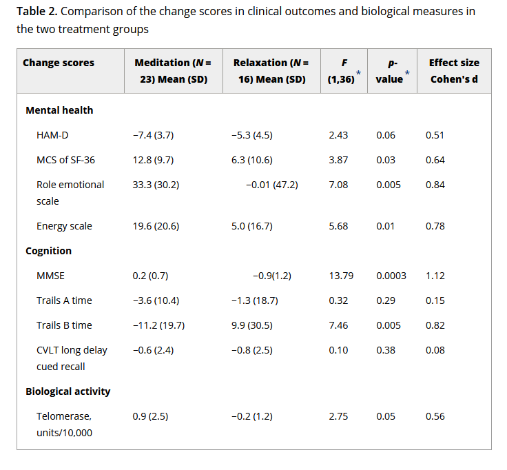
The third study gives us the mean and standard deviation of telomerase change over the course of the trial for each group. That is, they have subtracted each individual’s telomerase at baseline from their telomerase after the trial, and reported this difference. The mean and standard deviation of change score by group are related but not identical to the mean and standard of post-trial telomerase by group. The differences between the two group means are, in expectation, the same in the two cases. Since assignment is random, the expected value of the difference between the groups is zero at baseline, whereas after the intervention, the expectations of the two means differ by the expected value of change associated with the treatment. However, the standard deviation of change in telomerase within an individual over a few months is not really the same quantity as the standard deviation of telomerase across individuals.
Nonetheless, we are going to have to work with this. We are going to have to compare the group difference in post-trial telomerase for studies 1 and 2 with the group difference in telomerase change score for study 3. In my experience of meta-analysis, you have to make a constant series of small decisions like this in order to get anywhere at all, and often you are not exactly comparing like with like. Of course, it is much better if all studies openly archive their data in a repository. Then, you can go to the raw data and extract the exact same statistics from each one, in order to make your set of effect sizes more exactly comparable.
10.4.2 Extracting the data
So, we have some kind of mean and standard deviation of telomerase activity per group after the trial, and we have standard deviations of this within each group (of level, for studies 1 and 2; of change for study 3). This means that we can calculate an SMD value. We express the difference standardised (in terms of standard deviations) rather than in terms of actual units of telomerase activity per microlitre of blood, because the absolute numbers could be very different from study to study, for example if the lab equipment worked in different ways, the samples were prepared differently, and so on. By always comparing in terms of standard deviations observed within that study, you abstract away from these measurement differences.
To obtain the SMD, we need the means and standard deviations for each group, and also the number of participants in each group. Though these ns are not shown in the tables, they can be found in the three papers. Often, it’s quite hard to get the exact numbers, since some participants have missing data for some variables or time points, and the reporting is never quite as explicit as it could be. This is another reason for providing your raw data. Once we have identified the information we need, we start to make a data frame of the information from our three studies; something like this:
telo.data <- data.frame(
  studies = c("Daubenmier et al. 2012", "Ho et al. 2012", "Lavretsky et al. 2012"),
  mean.treatment = c(7.67, 0.178, 0.90),
  mean.control = c(7.51, 0.104, -0.2),
  sd.treatment = c(2.8, 0.201, 2.5),
  sd.control = c(2.5, 0.069, 1.2),
  n.treatment = c(19, 27, 23),
  n.control = c(18, 25, 16)
    )
10.4.3 Calculating the effect sizes
To calculate our SMDs, we need the contributed package we are going to use for our meta-analysis, metafor. Now is the time to install it if you don’t have it yet.
The metafor package has a function called escalc() which spits out effect sizes in various formats. We specify that measure="SMD" in calling escalc() to indicate that it is the SMD we want (the escalc() function spits out Hedges’ g, a version of the SMD with a correction for sample size) We have to tell the escalc()function to find the mean for each group, the sds for each group, and the ns for each group. Which group you select for group 1 here will determine whether your effect sizes will come out positive (i.e. a positive number when the treatment group is higher than the control) or negative (i.e. a positive number when the control group is higher than the treatment group).
telo.effect.sizes = escalc(measure ="SMD",
       m1i = telo.data$mean.treatment,
       m2i = telo.data$mean.control,
       sd1i = telo.data$sd.treatment,
       sd2i = telo.data$sd.control,
       n1i = telo.data$n.treatment,
       n2i = telo.data$n.control)
In your object telo.effect.sizes you should have the three SMD values in a column called yi, and their three sampling variances in a column called vi.
      yi     vi
1 0.0589 0.1082
2 0.4775 0.0792
3 0.5196 0.1094
It would be neater to put these into the original data frame telo.data, so let’s do this (cbind() binds two data frames with the same number of rows together into one).
10.4.4 Running the meta-analysis
Now it is time to fit the meta-analysis model, which we do with the function rma() from metafor. We specify where we want it to look for the effect size values yi and the sampling variances vi.
Random-Effects Model (k = 3; tau^2 estimator: REML)

  logLik  deviance       AIC       BIC      AICc
 -0.1420    0.2839    4.2839    1.6702   16.2839

tau^2 (estimated amount of total heterogeneity): 0 (SE = 0.0975)
tau (square root of estimated tau^2 value):      0
I^2 (total heterogeneity / total variability):   0.00%
H^2 (total variability / sampling variability):  1.00

Test for Heterogeneity:
Q(df = 2) = 1.2441, p-val = 0.5368

Model Results:

estimate      se    zval    pval   ci.lb   ci.ub
  0.3652  0.1796  2.0331  0.0420  0.0131  0.7172  *

---
Signif. codes:  0 '***' 0.001 '**' 0.01 '*' 0.05 '.' 0.1 ' ' 1
In the interest of transparency, you should get identical results by giving rma() the standard errors rather than the sampling variances:
So what does the model show? The estimate of 0.3652 means that our overall estimate, taking all three data sets into account, is that meditation has an effect of telomerase activity with an SMD of about 0.37, and a 95% confidence interval of 0.01 to 0.72. This confidence interval does not include zero, and so we say that the combined evidence is for a significant effect of meditation.
What else does the model tell us? The heterogeneity test (Q) is not significant and the heterogeneity statistic I^2 is estimated at 0%. These statistics mean, in effect, that the results of the studies do not differ any more from one another than would be expected given that they are extremely small, and small studies find variable results even when the underlying effect is constant. These heterogeneity statistics become more interesting in much larger meta-analyses, where studies may find quite different results depending on their methods or the populations they are done in.
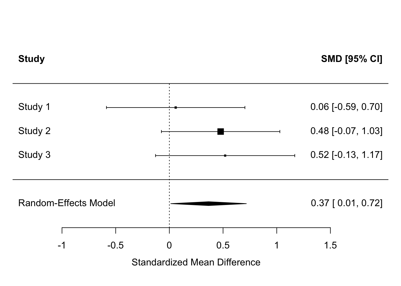
Now, let’s get the forest plot:
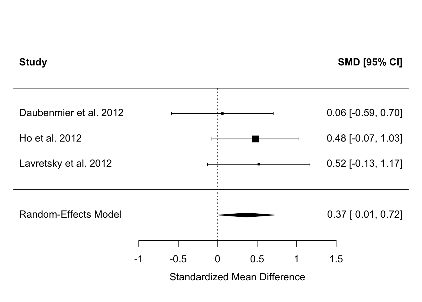
We can make it a bit nicer by telling the forest() function where to look for the names of the studies:
Although, by our simple analysis, none of the three studies has an effect estimate significantly different from zero, the results overall suggest there is an effect, whose best estimate is 0.37, with a 95% confidence interval from 0.01 to 0.72.
Something you might have noticed is that the claims about significance for the individual studies implied in the forest plot seem to be at odds with what the papers said. For example, Daubenmeir et al. reported no significant effect (and we concur), but both Ho et al. and Lavretsky et al. claimed their effects as significant, whereas we show their 95% confidence intervals as crossing zero. In both cases, this is because they performed more sophisticated analyses than our simple SMD, with more covariates, that make their precisions better. But, we had to use SMD since although it is basic we could get some version of it for every study. The point of meta-analysis is that the significance of individual studies is not terribly important; it’s the overall estimate that you are interested in, and in this, the overall evidence suggests that the claims Ho et al. and Lavretsky et al. made from their individual studies were probably generalizable.
10.4.5 Reporting the meta-analysis
I would report the results in something like the following way. ‘We combined the standardised mean difference estimates from the three studies and performed a random effects meta-analysis. The estimated overall effect size was 0.37 (95% confidence interval 0.01 to 0.72), suggesting evidence that meditation increases telomerase activity relative to control. There was no evidence for heterogeneity across studies (\(Q^2(2)\) = 1.24, p = 0.54; \(I^2\) = 0%). I would then show the forest plot. By the way, the default model fitted by metafor is a called a random-effects model. It assumes that the underlying effect sizes are drawn from a distribution whose mean we are trying to infer. There are alternatives (’fixed-effect models’), but I won’t go into them here as random-effects is more generally appropriate, and is more conservative.
10.4.6 Systematic reviewing
For this example, I just decreed that there were three studies in our set. How, in reality, would you establish the set of studies to include?
You would do so by systematic reviewing. In systematic reviewing, you perform a verifiable and replicable set of procedures to arrive at your set of candidate studies. Typically, this involves defining a set of search terms; using them to search online databases of scientific studies; screening the hits you found to determine which of these really meet the criteria needed to provide evidence on your question; then extracting the information from each one. Systematic reviewing is a whole discipline in its own right and I will not cover it in detail here. It often involves a lot of agonising about what a study really has to contain to constitute evidence on your exact question, rather than a related one.
The point, though, is that it is not sufficient to merely assert that there are three studies providing evidence on the question. Instead, you have to show that you made some kind of objective, thorough and replicable attempt to find all the evidence, and documented how you did that. Someone else should be able to repeat your systematic review and find the same sources.
An important part of a systematic review and metaanalysis is the PRISMA diagram. This identifies the steps in the reviewers’ workflow, showing exactly how the final set of included studies was identified and decisions about inclusion or exclusion arrived at. I encourage you to do a web search for ‘PRISMA diagram’ and see what one looks like. It gives you a good sense of how systematic reviewing works.
The combination of systematic reviewing and meta-analysis as an approach to evidence synthesis represents a major epistemological improvement in recent science. It is not without its problems, though. Just as in any individual study, there are many small judgement calls to be made in the process of doing a meta-analysis. Different researchers could make these differently, and hence come to different conclusions. Sometimes a whole field becomes convinced of something because of a meta-analysis whose results depended on very specific (and non-obvious) researcher decisions. In many areas there are now meta-analyses of meta-analyses! In any event, if you do meta-analysis seriously you should pay great attention to transparency, reproducibility, and sensitivity of conclusions to analytical decisions; just as is true for analysis of a single dataset.