11.4 Statistical power
Armed with our functions simulate() and hundred.sims(), it’s time to tackle the substantive topic of this chapter, statistical power. The statistical power of a test, given an effect size, is the probability that the test will detect that the effect is significantly different from zero, if in fact the effect is there. The investigation of statistical power is called power analysis. Our hundred.sims() function allows us to estimate statistical power for a given effect size and sample size in our planned experiment. The estimated power is simply the number of times out of the hundred that the result is significant.
We saw that with n=50 and effect.size=0.2, we usually don’t see a significant result. Let’s look at how the proportion of significant results changes as the true effect size gets bigger.
[1] "Effect size of 0.2"
Non-significant     Significant
84 16 [1] "Effect size of 0.4"
Non-significant     Significant
47 53 [1] "Effect size of 0.6"
Non-significant     Significant
15 85 [1] "Effect size of 0.8"
Non-significant     Significant
              3              97
As the effect size increases, the chance of detecting an effect significantly different from zero with n=50 gets bigger and bigger. You go from rarely doing so with effect.size=0.2 (power of around 20%) to almost always doing so with effect.size=0.8 (power of more than 95%). This gives us the first principle of statistical power: for a given sample size, the statistical power of a test increases with the size of the effect you are trying to detect.
How does varying our sample size impact our statistical power? I am sure you know that as your sample size gets bigger, your power gets better. Let’s try to visualize this. We will write a chunk of code that makes use of the hundred.sims() function to work out the estimated power with effect.size=0.2 for a whole series of different sample sizes, and makes a graph. The code will put the data into an object called power.sample.size.data. The comments help you understand how the code is working. It will take a few seconds to run. After all, this code is performing thousands of simulations.
# Try all the sample sizes between 10 and 600 in jumps of 10
# 'seq()' makes a sequence from the lower number to the high in intervals given by 'by'
Sample.Sizes <- seq(10, 600, by=10)
Power <- NULL
# Make a loop that will step through the Sample Sizes
for (i in 1:length(Sample.Sizes)) {
  # Do the current set of simulations for the sample size we are on
  Current.sim <- hundred.sims(n = Sample.Sizes[i], effect.size = 0.2)
  # Figure out the power at the sample size we are on
  Current.power <- table(Current.sim$Significant)[2]
  # Write this into the Power variable on the correct row
  Power[i] <- Current.power
  # Close the loop and moves on to the next sample size
}

# Record the data
power.sample.size.data <- data.frame(Sample.Sizes, Power)
Now, let’s make a plot of how power varies with sample size.
ggplot(power.sample.size.data, aes(x=Sample.Sizes, y=Power)) +
  geom_point() +
  geom_line() +
  theme_classic() +
  xlab("Sample size") +
  ylab("Power estimated through simulation")
You can clearly see the second principle of statistical power in operation: power to detect an effect of a given size increases as the sample size increases. Here it goes from less than 20% at sample sizes of less than 50 per group, to almost but not quite 100% with sample sizes of 600 per group.
On this graph, there is some noise in the power-sample size relationship. This is due to the fact that we only ran 100 simulations at each sample size. If you wanted to smooth this, you could run 1000 simulations at each sample size. This would give you much more precise estimates and a smoother curve, but it would take ten times as long to run.
You can probably also discern that the power gain from having more participants gradually flattens out. The power gain of going from 50 to 150 is bigger than the power gain of going from 450 to 550. This is because power generally increases with the square root of sample size. The simulations confirm this. Let’s see this by replotting the graph, but with a square-root transformation of the x-axis, and a straight line through the data.
ggplot(power.sample.size.data, aes(x=Sample.Sizes, y=Power)) +
  geom_point() +
  geom_smooth(method="lm") +
  theme_classic() +
  xlab("Sample size") +
  ylab("Power estimated through simulation") +
  scale_x_sqrt()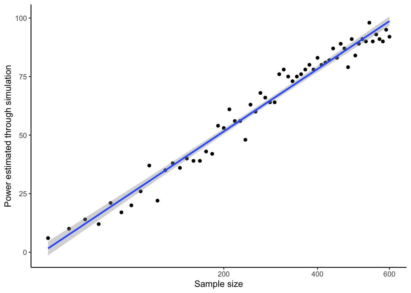
Why does power increase as sample size increases? We can investigate by looking at the histogram of the parameter estimates from a hundred simulations with different sample sizes, coloured by whether they were significant or not. Again, the comments help you see what the code is doing.
# Run 100 simulations at each of four sample sizes
h50 <- hundred.sims(n=50)
h150 <- hundred.sims(n=150)
h250 <- hundred.sims(n=250)
h350 <- hundred.sims(n=450)
Estimates <- c(h50$Estimate, h150$Estimate, h250$Estimate, h350$Estimate)
Significance <- c(h50$Significant, h150$Significant, h250$Significant, h350$Significant)
# Make a variable indicating the sample size
Sample.Sizes <- c(rep(50, times=100), rep(150, times=100), rep(250, times=100), rep(450, times=100))
# Put them in a data frame
Figure.data <- data.frame(Sample.Sizes, Estimates, Significance)
# Make the graph
ggplot(Figure.data, aes(x=Estimates, fill=Significance)) +
  geom_histogram(bins=10, colour="black") +
  theme_classic() +
  ylab("Number of simulations") +
  geom_vline(xintercept=0.2) +
  geom_vline(xintercept=0, linetype="dotted") +
  facet_wrap(~Sample.Sizes) +
  scale_fill_manual(values=c("white", "darkgrey"))
The reasons why larger sample sizes mean greater power are clear. In small samples, the parameter estimates vary widely from data set to data set. This is reflected in the large standard error of the parameter estimate, which means that the effects are rarely significant; in fact they are only significant where, by luck, the effect has been massively overestimated. As we move up in sample size, the variation in parameter estimate from data set to data set starts to be more modest; which means that more of them are significant, since the standard error is smaller relative to the typical parameter estimate. By a sample size of 450, almost all of the estimates are significantly different from zero. More crucially, by a sample size of 450, all of the parameter estimates that are around the true value of 0.2 are classified as significantly different from zero. The experiment with 450 participants per group looks adequately powered to detect a sample size of 0.2 standard deviations. The experiment with 50 or 150 group definitely is not; though, you might be adequately powered to detect much larger effects at these smaller sample sizes. Power is defined only for the combination of an effect size and a sample size.