6.2 Generalized Linear Models: Theory

In the General Linear Models we have examined so far, the mean of the outcome variable is related to the sum of the predictor variables, each weighted by the relevant parameter estimate (this right-hand side part of the model is called the linear predictor). Where we have just one predictor variable, then, the model is as follows (see section 3.3):

\[ E(Y) = \beta_0 + \beta_1*X \] What though if our outcome variable is not continuous? Consider the case where the outcome variable is an event that either happens or does not (i.e. is binary, with 0 representing the outcome not happening and 1 representing the outcome happening). Here, the model above does not fit the situation too well. If you look at the linear predictor part in the equation, \(\beta_0 + \beta_1 * X\), it implies that as \(X\) gets bigger, then the expected value of \(Y\) will get bigger too, in a straight-line fashion (assuming \(\beta_1\) is positive). There is no upper limit to this assumed linear relationship; for any value of \(X\), adding a further 1 to it will cause the expected value of \(Y\) to get bigger, by an amount \(\beta_1\). If the outcome variable is an event, its expectation can’t go on getting bigger indefinitely as the predictor variable gets bigger. The probability of \(Y\) happening is bounded at 1 (and at 0), so a linear relationship between the value of \(X\) and the expected value of \(Y\) extending indefinitely in both directions is not a defensible assumption.

In Generalized Linear Models, the linear predictor on the right-hand side is as before, but the outcome on the left-hand side is not the \(Y\) itself, but some function of \(Y\). That function is called the link function. Let’s call the link function \(f\). Then the model looks like this: \[ f(E(Y)) = \beta_0 + \beta_1*X \]

Written like this, we can see that our familiar General Linear Model is just the case of the Generalized Linear Model where the link function is the identity function \(f(E(Y))=E(Y)\). Generalized Linear Models come in many types, which are organised into families depending on the type of link function that they use.

What link function might we choose instead for the case where \(Y\) is binary? The most common choice is the logit function: \[ logit(p) = log(\frac{p}{1-p}) \] Here, \(p\) is the probability of the outcome event happening. Why is the logit function suitable? Here is how the implied value of \(p\) behaves as the value of the linear predictor changes under the assumption of a logit link function.

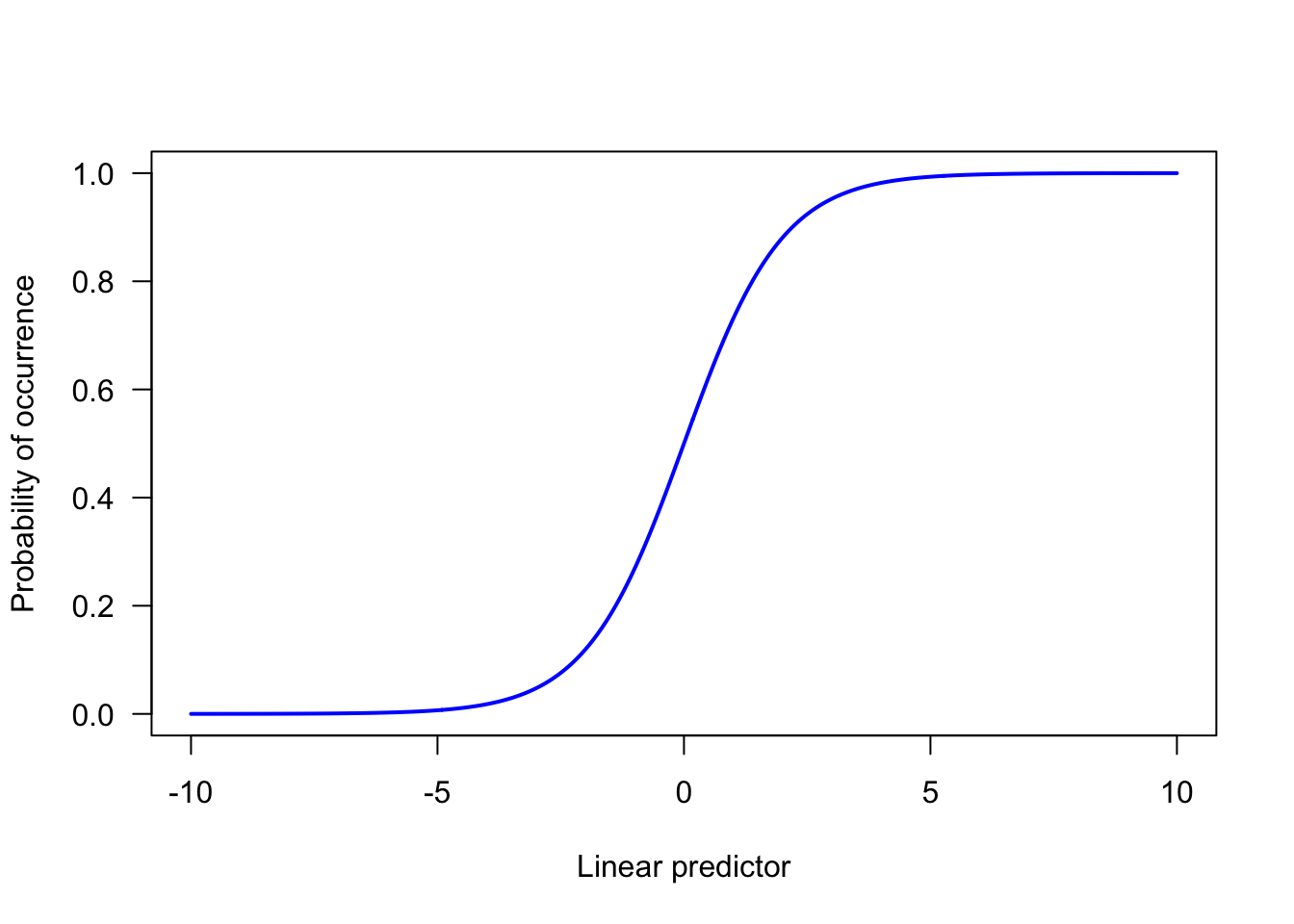
As you see, as the linear predictor gets large in the positive direction, \(p\) asymptotes at 1; the outcome is certain to happen. As the linear predictor gets very negative, \(p\) asymptotes at 0; the outcome is certain not to happen. And in between, there is a zone where \(p\) gets bigger as the value of the linear predictor gets bigger: by implication, the outcome event becomes more likely as the value of the predictor variables changes.

A Generalized Linear Model with a logit link function is known as a logistic regression model, a model of the Bernouilli family, and a model of the binomial family (these terms are not exact synonyms - each one denotes a successively slightly larger class of models - but for our purposes they are near enough). The treatment so far has been a bit abstract; Generalized Linear Models are actually quite easy to work with in R. Let’s turn to an empirical example.