3.2 Fundamentals of inferential statistics
Before turning to our first General Linear Model, we need to establish the logic of what inferential statistics is about, using a very simple hypothetical case.
3.2.1 Samples and populations
We generally work with modest samples of participants or observations. Say I am doing an opinion poll for an upcoming referendum. I might ask 2000 people which way they are going to vote. This sample is a kind of small world. We don’t really care about the small world per se, though. We care about the large world of which the small world is a studiable part. In the opinion poll case, I care about how the 30 million voters will vote on referendum day; the 2000 in my sample of mainly of interest because they can give me some information about that larger world.
The large world from which your sample is drawn in called the population. It is almost always impractical to study the whole of the population (the rare exception is things like censuses, which are supposed to contain the whole population of interest, not just a sample). Indeed, the idea of studying the whole population does not even make sense in many cases: for example, if you are studying the functions of some area of the human brain, the population of interest is the brains of all current humans plus those who have not yet even been born. So you study a small world, a sample, and try to extrapolate to what might be true about the large one from the data you get. Of course, this raises questions about the extent to which your sample is representative of the population you wish to make inferences about. We won’t go into these questions here, but your inferences are only secure for that population which is like your sample in terms of the parameters specified in your model.
3.2.2 Models, parameter estimates, and confidence intervals
The first step in inference is to write down a statistical model of the situation you want to understand. This model contains parameters, often denoted with Greek letters. These parameters are properties of the population (not the sample), and their value is, by definition, unknown.
In the case of our opinion poll, the model is as simple as can be:
- A proportion \(\theta\) of the population intends to vote ‘Yes’ on referendum day.
In the terms of chapter 1, the parameter \(\theta\) is our estimand. How then are we going to figure out what its value is? It turns out, through some maths I won’t go into, that as long as my sample is representative of the population from which it is drawn, the best possible estimate of the unknown parameter \(\theta\) is just the proportion of my sample who said they intend to vote ‘Yes’. Thus, if I sample 2000 people and 54% of them say they intend to vote yes, then my best parameter estimate for \(\theta\) is 0.54.
But, my parameter estimate is imprecise. I could be a bit wrong. I could have got lucky or unlucky in who happened to fall into my sample. The magnitude of this imprecision is going to depend on my sample size (the number of people I interview). To see how this might go, the figure below simulates 100 data samples drawn from a population where \(\theta\) really is 0.54. For a series of sample sizes between 5 and 2000, I plot what my parameter estimate would be if I stopped sampling at that sample size.
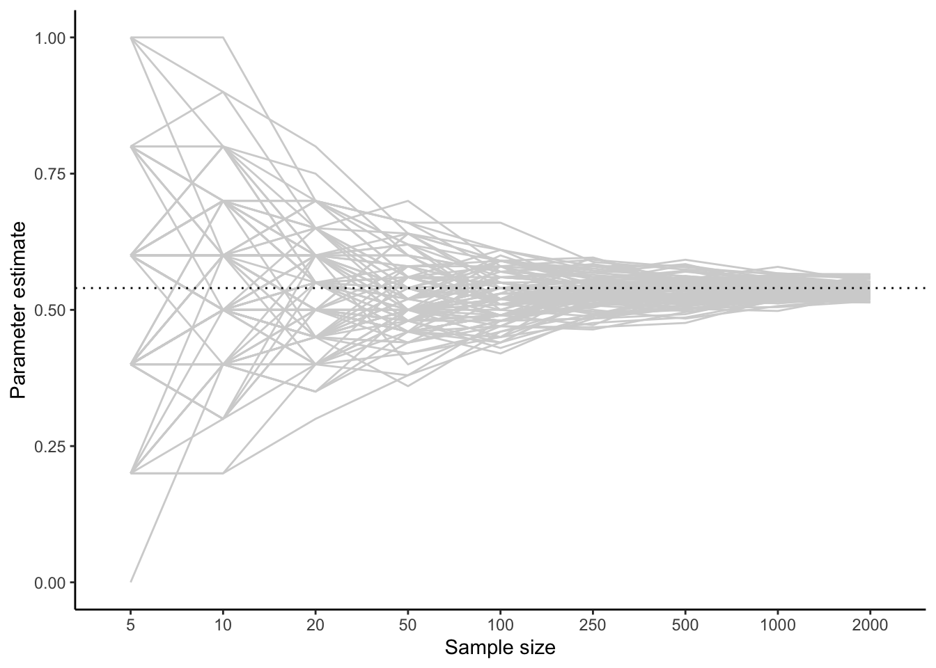
You can see that on average, and regardless of sample size, I get an answer of 0.54 (this is good!). However, I get some variation from sample to sample. With small sample sizes, this variation can be dramatic: I can have estimates of \(\theta\) as small as zero or as big as one. The larger my sample size, the more narrowly my estimates cluster around 0.54, though even with 2000 respondents, my achieved estimate varies a bit from time to time.
Thus, any parameter estimate from any study is imprecise to some extent, because of our finite sample size. We characterize this imprecision in two related ways. The first is the standard error of the parameter estimate. This can be thought of as ‘the amount by which a typical parameter estimate might be wrong either way’. The second is the 95% confidence interval for the parameter estimate. This is the interval within which, were you to run your study 100 times, 95 of your realised parameter estimates would fall. The choice of 95 is arbitrary but conventional; you could just as well report an 89% confidence interval, or a 99% confidence interval. When you report a parameter estimate, you should always report either the standard error or the 95% confidence interval, to give your reader a sense of the margin of error of your inferences.
You may be wondering how you are supposed to know the standard error or confidence interval of your parameter estimate. After all, you don’t know the true value of the parameter (that’s the whole point), and you aren’t going to run your study 100 times. Suffice it to say that there are some mathematics we won’t go into that estimate these things, based on the observed variability in the data, and your sample size. R spits them out for you. The standard error and confidence interval are related: in simple cases, the 95% confidence interval is your observed parameter estimate plus or minus 1.96 times the standard error.